Value for Money and the Public Sector Comparator

Manual M1 · Austral Manual Series

Download PDF ↓Versión en españolVersão em portuguêsVersion française

Valor por Dinero y Comparador Público‑Privado — Manual M1 de Austral

Version 1.1 · 16 September 2026 (version 1.0: 14 September 2026)
Austral Intelligence · David Duarte Arancibia, with Mika (Austral's analysis agent)
Platform module that runs the method: Value for Money (/vfm) — PPP Value‑for‑Money Analyzer
Languages: English (this edition), Spanish, Portuguese and French · HTML and PDF at austral‑intelligence.com/manuals

Abstract

This manual explains how to decide, with defensible numbers, whether an already‑approved infrastructure project should be procured as a public‑private partnership (PPP) or through traditional public works. It presents Value for Money (VfM) analysis and its instrument, the Public Sector Comparator (PSC), as a self‑contained thirteen‑step method, each step with its inputs, outputs, computation and decision rule; traces every rule to the international guidance that set it and says where the sources disagree — in particular on the discount rate, where the manual adopts two rates by branch, the government's risk‑free rate plus a spread for the systematic risk each branch bears, and declares this as a decision; walks the thirteen steps through a generic regional hospital procured under an availability payment, with every figure shown; shows how the method runs on the Austral platform, screen by screen; and explains why this particular method breaks in a spreadsheet. It is written for PPP units, ministries of finance and auditors.

How to cite

Austral Intelligence (2026). Value for Money and the Public Sector Comparator. Manual M1, Austral Manual Series, version 1.1, September 2026. https://austral-intelligence.com/manuals/value-for-money/

A note on the figures

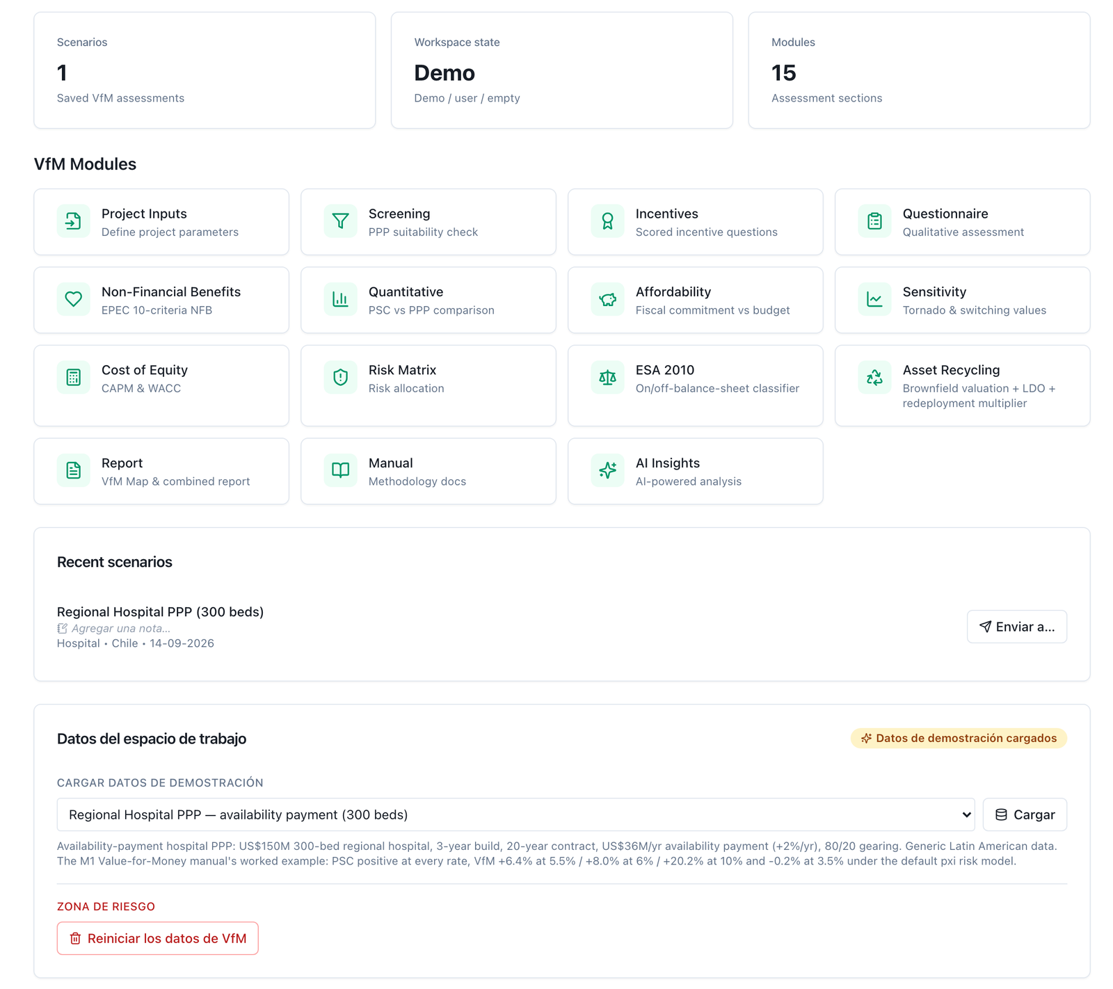
Every figure in the worked example (section 4) and in the screenshots (section 5) is generic: it belongs to a hypothetical 300‑bed hospital shipped as a demonstration pack in the platform, calibrated so that the method can be followed from start to finish. None of it comes from a client or from a real project, and none of it should be used as a reference for the costs, payments or risks of any actual project. The tool's default values (marked ◆ in the text) are Austral calibrations, configurable in every scenario, and are published so that a reviewer can challenge them. The methodologies cited are credited to their authors; the only product name in the manual is Austral.

Version 1.1 change note

Version 1.1 (16 September 2026) replaces the single discount‑rate rule of version 1.0 with the two‑rate rule by systematic risk: each branch is discounted at the government's risk‑free rate plus a spread for the systematic risk it bears — zero in the public comparator, the transferred share in the PPP — with the bands from the Australian guide (National PPP Guidelines, vol. 5) cited as a reference, and a rule against double counting: project‑specific risk is priced into the cash flow and systematic risk into the rate, never both. This changes the reading warning and the comparison table in section 2, steps 5, 8 and 10 and the checklist in section 3, the example in section 4 — recalculated at two rates, with the single‑rate reading alongside — the screens and exports in section 5 (rate card, the nature of each risk, the unbundled tornado chart, the rate convention in the report and the workbook), and the mentions of the single rate in sections 1 and 6. The base case's risk‑free rate is the government bond at spot — real BTU‑20, 2.70%, 18‑08‑2026, Central Bank of Chile — with its provenance; the 2016–2025 average for the same bond (1.85%) remains as a sensitivity, under which the example reads as marginal rather than positive. The Peruvian reference (Law 32441 of 2025) and the citation of the Australian guide, with its exact sections, are also corrected.

Contents

1. What it is for and when it is used
2. International methodological basis
3. The method, step by step
4. Worked example: a regional hospital under an availability payment
5. Implementation on the Austral platform
6. Why not in Excel, for this method
7. References and further reading

1. What it is for and when it is used

A ministry has a project it has already decided to build —the country needs the hospital, the road, the prison— and one question left: how to procure it. It can tender the works and run the asset on the public budget, or hand a private partner the design, construction, financing and maintenance for twenty or thirty years in exchange for a payment. Value for Money (VfM) analysis exists to answer that question with numbers, and to make the answer defensible before whoever approves it and whoever audits it three years later. Its central instrument is the Public Sector Comparator (PSC): the cost to the State of delivering the same service, to the same standard, through traditional public works.

1.1 The question it answers — and the one it does not

The VfM question fits on one line: does it cost the State less, adjusted for risk, to do it as a public‑private partnership (PPP) than through traditional public works, for the same service?

Every word does work. The State: what is compared is the Treasury's outlay, not the profitability of the business nor the welfare of the user. Adjusted for risk: cost overruns, delays and maintenance failures have an expected value, and that value is added to whichever leg bears them; the heart of the method is that a PPP saves the State the risk it transfers, and charges for it. For the same service: the public option has to deliver the same hospital, to the same standard, with the same maintenance; if it is modelled cheaper because it is assumed worse, the comparison loses its meaning.

From that follows what VfM does not answer. It does not say whether the project is worth doing —the socio‑economic appraisal decided that, earlier, with a different metric. It does not say whether the State can pay for it: a contract can be the cheapest procurement route and still commit more annual budget than the sector has.

What VfM is not

• It is not a social appraisal. It does not measure benefits to the population or a social return. That test comes first and, if the project fails it, VfM should not be computed at all.
• It is not an affordability test. A positive VfM does not make a project payable. The annual payment profile against the budget ceiling is a separate, later test, and it can reject a contract with positive VfM (step 12 of the method).
• It is not a grade for the project. It compares two ways of procuring the same thing: a bad project with high VfM is still a bad project, procured the cheapest way.

1.2 Where it sits in the project cycle

VfM has a precise place, and it arrives late: it is not the project's first test but one of the last before tendering.

Before it come two gates. The socio‑economic appraisal, which decides whether the project is done at all. And the PPP eligibility screen —eight yes/no questions: need, output‑specifiable service, size, legal framework, transferable risks, measurable service, institutional capacity, market interest— which decides whether the project is even a PPP candidate. A "no" there is not offset by a good number: it is resolved, or the project goes the traditional route. (It is the screen of the PPP Eligibility Index, manual M3 of this series; the method applies it at step 1.)

First computation: ex ante, before tendering. With the project approved and declared eligible, VfM compares the risk‑adjusted PSC with the estimated cost of the PPP and produces two things the tender documents need: the verdict that authorises —or not— structuring the project as a PPP, and the reserve price, the maximum payment at which the PPP remains as cheap as public works. Without that second number, an ex ante VfM binds nobody to anything.

Second computation: with the awarded bid. Once the tender is awarded —the moment the State knows the real price before it commits— the same computation is redone with the payment of the awarded bid in place of the estimate, and with the same rate convention —the same risk‑free rate and the same spreads—, the same risk register and the same scales as the ex ante analysis. What matters is the reconciliation: how much of the difference came from the bid price, how much from a change in allocation, how much from an input correction. Without that reconciliation the second VfM confirms nothing about the first; step 13 of the method sets out how it is done.

What is not appropriate is the third use, the most frequent in practice: computing VfM after deciding, to confirm the decision. A comparator built to support a conclusion already reached always supports it; section 6 shows how easily.

1.3 Who uses it and for what

Four readers, four different uses of the same computation.

• The PPP unit, to structure. It builds the PSC and extracts from it the reserve price and the risk allocation to be written into the contract. VfM also tells it where the value comes from: if all of it comes from transferring construction and life‑cycle risk, the deduction regime and the rebalancing triggers stop being fine print.
• The Ministry of Finance or the budget office, to approve and to account for the liability. It receives the verdict and, above all, the annual payment profile: the firm commitments that go into its register and the guarantees that go into the contingent‑liability register (the subject of manual M2 of this series). It is also the one that sets the parameters of the discount rate —the government's risk‑free rate and the band for the systematic‑risk spread of each branch—, which are policy and not a project output.
• The audit office, to review. It does not recompute the project: it verifies that the computation can be reconstructed —rate convention with the risk‑free rate and the spreads, and their sources, published scales, no risk counted at once in both the cash flow and the rate, seed and number of runs of the simulation, verdict with its band, sign of the comparator. Section 3 closes with that list.
• Bidders, to anticipate. A published PSC tells the market what payment ceiling the State considers defensible and which risks it expects to transfer: it improves bids and reduces surprises at evaluation.

1.4 The four possible results

The method produces VfM in money and, where it applies, as a percentage of the comparator. The verdict has four readings, not three, and the fourth is the one almost no report documents.

• Positive. The PPP costs the State less, risk‑adjusted and for the same service, by a margin that exceeds the model's noise and survives the sensitivity analysis: it authorises structuring as a PPP, with whatever conditions the analysis identifies.
• Marginal. The difference exists but sits inside the estimation error of the inputs themselves; it is not a tie in the PPP's favour but an obligation to look at the switching values before deciding.
• Negative. Traditional public works are cheaper: the best service VfM renders is to avoid a thirty‑year contract nobody would have defended afterwards.
• Not interpretable. When the adjusted comparator is not a positive net cost —typically in a self‑financing project, one the State would operate at a profit— the percentage is a ratio whose denominator has changed sign, and it stops saying what it seems to say. VfM is reported in money, the rate is declared and the case is reviewed; the percentage is not quoted and no banded verdict is issued.

Over those four sits the qualitative axis: a positive VfM with a failed eligibility screen is not a positive result, it is a conflicting one. The exact bands, the crossing with the qualitative axis and the decision map are in step 9 of the method (section 3).

1.5 What the manual delivers

Three things, in this order.

A self‑contained method. Section 3 develops the thirteen steps of the analysis —from the frame and unit of account to the bid VfM— with what goes in, what comes out, how it is computed, what the decision rule is and where teams usually go wrong. It is written to be run with any tool, a spreadsheet included. Section 2 traces every rule to the guidance that set it —the World Bank's PPP Reference Guide, HM Treasury's Green Book, PFRAM 2.0 and the national comparator guidelines— and says where the sources disagree with each other.

A reproducible example. Section 4 walks the thirteen steps through a generic regional hospital procured under an availability payment —US$ 36.0 M a year— with every figure and the result of each step: VfM of +5.9% of the comparator with the PSC at the government's risk‑free rate (2.70% real, the 20‑year bond spot rate) and the PPP at that rate plus a 0.9% spread for the transferred systematic risk, positive by a small margin, +3.5%, marginal, if the risk‑free rate were the ten‑year average of the same bond (1.85%), and +6.5% at a single real rate of 5.5%, positive, with its fragilities declared. It is not a showcase case, and that is why it teaches: the value lies entirely in the transfer of construction and life‑cycle risk, and the verdict changes band with the risk‑free rate chosen within the range the same bond has shown over ten years.

The tool that runs it, and that the client keeps. Section 5 shows how the method runs on the Austral platform, screen by screen, and what the exports print. Section 6 explains why this particular method —not any computation— breaks in a spreadsheet, with the failures measured on the same hospital. Section 7 gathers the references with their verification status.

A reader who only wants to know whether a VfM report that lands on their desk for signature was done properly can go straight to the reviewer's checklist at the close of section 3.

2. International methodological basis

Every rule of the method in section 3 comes from a guideline that a ministry applies or once applied. This section says where each one comes from, with section or paragraph, so that a reviewer can argue the rule at its source and not in the manual. Three primary sources set the frame (the World Bank's PPP Reference Guide, HM Treasury's Green Book and PFRAM 2.0); five national Public Sector Comparator (PSC) guidelines set the practice; the Latin American cases show where countries part ways with each other. Table 2.7 links every step of section 3 to its source and to the screen of section 5 that runs it.

Reading warning: the sources agree on the architecture of the PSC and on the fact that project‑specific risk is valued in the cash flow, not in the discount rate. They do not agree on which rate to use, or on whether both legs are discounted at the same rate: HM Treasury, EPEC and South Africa mandate a single rate for all options; the Australian guideline mandates different rates per leg, each equal to the government's risk‑free rate plus a spread for the systematic risk that leg bears. The manual adopts this second position —two rates for systematic risk, declared with their provenance— and presents it as a decision, not as a consensus; Table 2.4b summarises what each guideline does, and §2.6 states where the manual departs even from the Australian guideline.

2.1 The World Bank PPP Reference Guide, version 3 (2017)

The PPP Reference Guide, Version 3 (World Bank, ADB and IDB, 2017), module 3 "PPP Cycle", §3.2 "Appraising Potential PPP Projects", evaluates a PPP candidate against five criteria: project feasibility and economic viability (§3.2.1), commercial viability (§3.2.3), value for money (§3.2.4), fiscal responsibility (§3.2.5) and the capacity to manage the project (§3.2.6); environmental and social studies sit in §3.2.2. VfM asks whether "developing the project as a PPP can be expected to achieve the best value for money compared with other options", public procurement included (§3.2).

§3.2.4 distinguishes three families of method, which section 3 uses in that order: qualitative VfM —is the project of the kind that private capital should finance, and are the conditions for a PPP to create value in place?— with HM Treasury's suitability criteria as the example (step 1); the quantitative PSC, "the most common quantitative tool", which compares the fiscal cost of both routes before tendering, against a "shadow PPP", and during tendering, against the actual bids (steps 4–9 and 13); and the economic cost‑benefit comparison, which hardly anyone practises and this manual does not develop. Box 3.5 sets the two adjustments that make the PSC comparable —risk and competitive neutrality— and requires "defining the appropriate discount rate for the cash flows of both the PPP model and the PSC". The Guide also records the criticisms of the PSC, among them "the possibility of manipulation to reach the desired conclusion": that risk is the reason for section 6 and for the discipline of step 8. And it notes that Colombia and Peru wrote PSC guidelines but "neither has implemented the full methodology in practice" (§3.2.4).

2.2 HM Treasury's Green Book (2026) and its optimism‑bias guidance

The current edition of the Green Book is that of February 2026, which replaces the 2022 edition. Three rules of section 3 come from it.

One rate, and which one (the rule this manual does not follow). §6.54 sets the social time preference rate (STPR) at 3.50 % real for years 1–30, 3.00 % for years 31–75 and 2.50 % from year 76; §6.56 requires it to be applied to real values, without adding inflation. Annex A, on private‑finance models, is the direct source of the rule: the shortlist "should typically include a public sector option" (§A.10) —"also known as a public sector comparator" (§A.13)—, all options are discounted at the STPR and a sensitivity in which the costs of all options are discounted at the risk‑free gilt rate is mandatory (§A.17–A.18). Never one rate per leg. It is the rule followed by most guidelines, and the one the method admits as an alternative convention (step 8); the manual replaces it with the Australian rule (§2.4 and §2.6) and retains from it the mandatory sensitivity to the risk‑free rate, which in step 10 becomes the variable that is moved.

Risk by expected value, optimism bias explicit. §6.69 admits the expected value as the central estimator and §6.67 includes contingent liabilities in the expected cost of risk. §6.79–6.82 require adjusting for optimism bias from the outset —costs and durations upwards— with the appraiser's own historical evidence or, failing that, the generic values of the supplementary guidance, and reducing the adjustment in proportion to the risk mitigated. §A.14 applies the adjustment "to all options on the shortlist" and corrects, in the public option, the differences in effective tax burden: the competitive neutrality of step 6.

The reference uplifts. The Supplementary Green Book Guidance: Optimism Bias (HM Treasury; on GOV.UK since 21 April 2013; basis: Mott MacDonald, 2002), table 1, upper / lower bound on capital expenditure: standard buildings 24 / 2 %, non‑standard 51 / 4 %; standard civil engineering 44 / 3 %, non‑standard 66 / 6 %; equipment and development 200 / 10 %; outsourcing 41 / 0 % (on operating expenditure). One "always starts from the upper bound" (§3.11) and reduces for mitigation (§3.12–3.14). It is the reference for the legacy model of step 5; the table by type of works and by risk on the risk screen is Austral's own disaggregation, and the manual says so.

The history matters: the Treasury's Value for Money Assessment Guidance (2004, updated November 2006) shaped the PSC of the PFI era; the Treasury withdrew its quantitative tool on 5 December 2012, and the model discounted both legs at the STPR (3.5 % real, 6.09 % nominal), so that it "only measured the cost of private finance above the social rate" (NAO 2013, summary §7 and §3.15). The 2026 gilt‑rate sensitivity answers that criticism.

2.3 PFRAM 2.0 (IMF–World Bank, 2019): the fiscal frame in which VfM has to close

The PPP Fiscal Risk Assessment Model 2.0 (manual, September 2019) was developed jointly by the IMF and the World Bank; Austral's founder took part in its development from the World Bank team. First, what PFRAM does not do, in the words of its manual: it does not "determine the procurement option (PPP versus traditional public investment)", because it "does not investigate the implications of the same project under traditional procurement" (§II.B). PFRAM does not compute a PSC. It supplies the frame in which the result has to close:

• the fiscal dimension of the PPP leg (§III.C): availability payments and capital grants as firm commitments; debt and minimum‑revenue guarantees as contingent liabilities, measured by maximum exposure and by expected payments under shock. Step 12 uses that separation;
• the accounting treatment (§III.D): PFRAM applies IPSAS 32 —asset and liability on the government's balance sheet if the government controls the service and the residual interest, whether the government or the user pays— because it "removes the accounting bias in favour of PPPs", so that a PPP is undertaken "for its own added value" and not "because it can be kept off the books" (box 2); the difference from the GFSM 2014 risks‑and‑rewards test is "more theoretical than practical". That is why VfM is a cost test, not a way of taking debt off the balance sheet;
• the fiscal risk matrix (§III.E and annex I): eleven categories and 52 sub‑categories, with likelihood and impact on three levels and a severity rating. The register of step 5 simplifies it to nine risks by phase plus renegotiation, with the same probability × impact logic and published numerical scales.

2.4 The PSC guidelines that set the practice

Australia — National PPP Guidelines, vol. 4, Public Sector Comparator Guidance (Dec. 2008) and vol. 5, Discount Rate Methodology Guidance (Aug. 2013). Vol. 4 is the canonical anatomy: "PSC = raw PSC + competitive neutrality + transferable risk + retained risk" (§2.3), with risk valued "in the numerator of the cash flow" as "consequence × probability + contingency factor" (§6.2). Vol. 5 is the source of the method's discount‑rate rule (step 8), and the only national guideline that formulates it: "only systematic risk is reflected in the rate" —project‑specific or diversifiable risk "is not recognised in the discount rate" and goes "into risk‑adjusted cash flows" (§2.4)—; four rates (§1.4): the risk‑free rate (long‑term government bond), the project rate (all systematic risk borne by the private party), the PSC rate (the risk‑free rate, because under public provision the State retains all systematic risk) and the PPP rate (risk‑free rate plus the share of systematic risk actually transferred); a modified CAPM that builds it —project premium = asset beta × market premium, 6 % "consistent with Australian regulatory practice" (§2.9, §4.4)—; a beta range of 0.3 to 0.8 for social infrastructure under availability payments (§3.3, table 2) and a table that allocates the premium according to the share of each systematic risk transferred (§3.5, table 4); to "do I evaluate the bids at the same rate?" it answers "No" (appendix F). Its worked case is a hospital in New South Wales: beta 0.45 → premium 2.7 %; demand 90 % and residual value 100 % retained by the State, inflation 40 % and insolvency 90 % transferred → 0.92 % over the risk‑free rate (appendix C). For a toll‑road project it reverses the pair: the PSC, which bears all demand risk, uses the project rate, and the PPP's payments use the risk‑free rate (appendix D). It is also the guideline with the most real PSCs behind it and the one Chilean comparators take as their reference. Two of its choices that the manual does not copy, and which §2.6 declares: the guideline keeps the expected value of every risk, systematic or not, in the PSC cash flow and reserves the spread for the premium on variability (§1.6, §2.5); and it prefers a nominal, current risk‑free rate (§4.3).

South Africa — National Treasury, PPP Manual, module 4, PPP Feasibility Study (2004). Skeleton of the step 5 register: stage 4, part 2, builds the risk‑adjusted PSC in eight steps, and step 4 sets the rule: "the Treasury advocates costing risk as a separate line in the cash flow, not by adjusting the rate", multiplying cost by the likelihood of each sub‑risk with its timing. It prescribes no rate —a government bond of similar tenor, a premium only "where it is not possible to reflect all risks in the cash flow"— and requires it to be applied "consistently across all models" (stage 4, part 1).

Ontario — Infrastructure Ontario, Assessing Value for Money (Mar. 2015). Each risk with three points (probability and impact at the 10th percentile, "most likely" and 90th, as % of base cost), valued at the mean and not at the "most likely", precisely against optimism bias (risk annex, step 3). VfM is computed at structuring and again at award, with the real financing of the preferred bid (§2 and §4): step 13. Both legs at the province's cost of borrowing (§4).

United Kingdom. Seen in §2.2: mandatory public option, the same STPR for all options, gilt‑rate sensitivity, tax neutrality and optimism bias in all (annex A).

Europe — EPEC, Value for Money Assessment: Review of Approaches and Key Concepts (EIB, Mar. 2015). Its §2.3 says what section 3 repeats: risk goes in the cash flow or in the rate, "but it is important to avoid double counting", and "in most cases the same discount rate is applied to the cash flows of the conventional procurement and of the PPP option". Its note on non‑financial benefits (EPEC, Jun. 2011) is the source of the third score of step 2. Normative close: the OECD Recommendation on the governance of PPPs (4 May 2012) asks that the investment decision be taken separately from how it is procured, "without any institutional, procedural or accounting bias either in favour of or against PPPs" (principle 4), that it be investigated "which investment method is likely to yield most value for money" (5) and that each risk be transferred to whoever bears it at least cost (6); its principles 10–11 —affordability and disclosure of costs and contingent liabilities— are the mandate of step 12.

Table 2.4b — The discount rate, guideline by guideline, and the manual's position. This is the point where the sources do not agree, and it is therefore shown separately.

One‑line rationale: the State bears systematic risk at its own rate —the risk‑free rate— and the private party charges for it in the price; discounting both legs at the same rate ignores that the PPP transferred (and pays for) part of that risk, and discounting the PPP at the partner's WACC charges the project‑specific risk already in the payment in the rate as well. The Australian rule is the only one on the list that puts into the rate exactly what the rate remunerates, and the manual adopts it with a declared adjustment.

2.5 Latin American practice

Chile. There is no published official PSC guideline, and the report cited below invokes no rule requiring one. The public case is the Comparador Público Privado para el Centro Penitenciario de Rancagua (DIPRES, August 2024). Its §4 defines the method in the terms of this manual —a risk‑adjusted public reference project against the cost of the PPP, retained risk on both legs—, cites the Australian volumes 4 and 5 and Uruguay's CND methodological guideline, and takes a decision worth underlining: it acknowledges that the Australian guideline would lead to discounting the PPP leg at a higher rate, but discounts both legs at the same risk‑free rate, 6 % real, that of the National Investment System when the study was prepared (§5.4). Result (§5.5, table 27): public base cost 2,806,598 UF plus transferable risks 946,137 UF, against 2,697,368 UF of PPP payments and administration; VfM of 1,055,367 UF, 28 %, over 15 years. The social rate in force today is 5.5 % real (Precios Sociales 2026, MDSF, table 1.1): the cut from the 6 % DIPRES used was proposed by the update study of the Social Investment Evaluation Division (31 May 2024) and has applied since Precios Sociales 2025 (March 2025). Box 4.11 reads the case with the method.

Mexico. The most codified practice: article 14, section IX, of the Ley de Asociaciones Público Privadas requires the convenience analysis, governed by the SHCP Lineamientos (DOF, 31 December 2013) and its Manual (2012). The PSC of the Paquete Sureste (BANOBRAS for FONADIN, May 2020): total risk 4,178.6 million pesos, 1,744.9 retainable and 2,433.7 transferable, allocated risk by risk in its table 7; real risk‑free rate of 30‑year Udibonos, 3.93 % in March 2020, for both legs.

Colombia. Law 1508 of 2012 created the regime; the DNP set the parameters in Resolution 3656 of 2012, whose annex was replaced by Resolution 857 of 2023. Distinctive feature: the PSC is discounted at the project WACC (Ministry of Finance methodology, Res. 2080 of 2008) —one rate, but a market one (2012 annex, §2.7; 2023 annex, §3.3.1)—, while the social appraisal uses the DNP social rate, 9 % effective annual real (Resolution 1092 of 2022, art. 1).

Peru. Legislative Decree 1012 (2008) required a "comparative analysis" (art. 8.1), with a methodology approved by Ministerial Resolution 249‑2014‑EF/15 and progressive application by sector. The later regime (LD 1224 of 2015 and LD 1362 of 2018) replaced it with qualitative eligibility criteria, and Law 32441 (El Peruano, 16 September 2025), which repeals LD 1362 and, with its regulations (DS 316‑2025‑EF), governs today, preserves that architecture: the value‑for‑money principle of its article 4.2.1 —"the optimal combination between costs and the quality of the public service", with "an adequate distribution of risks"— is achieved, among other means, by "selecting the most suitable delivery modality … taking into account the application of the eligibility criteria", and for regional and local governments article 40.2 requires a "preliminary analysis of the benefits" of the PPP "compared with the public‑works modality, based on the criteria set out in the Regulations". The MEF's Guidelines for the application of the eligibility criteria define themselves as "a qualitative methodological instrument for analysing the value‑for‑money principle". The general social rate of Invierte.pe is 8 % real (Directive 001‑2019‑EF/63.01, annex 11). It is the case the Reference Guide describes: guidelines written, full quantitative methodology never applied.

Where they part ways, on two axes. The rate: the country's risk‑free rate (Chile 6 %, Mexico 3.93 %), the project WACC (Colombia) or the social rate (Chile 5.5 %, Colombia 9 %, Peru 8 %); every public case applies one rate to both legs —none has yet followed the Australian route this manual adopts, and Rancagua expressly rejects it—. Risk: expected value in the cash flow with a register by category in all three cases, with varying depth in the risk‑by‑risk allocation, where the Mexican PSC is the most explicit. The method of section 3 is compatible with all three: the rate convention (one or two) is an input declared with its source, the single‑rate reading is kept as a comparison, and the register is published with its scale and with the nature of each risk.

2.6 What Austral adds and cites as its own

The house frame is in The Optimal Risk‑Retention Frontier (Austral, 2026, §6). Its thesis, in one line: the contribution to VfM of transferring a risk is M − P, the management gain the private party obtains minus the premium it charges for bearing it. For a controllable risk (design, construction, operation) M exceeds P and the transfer creates value; for a macro risk (aggregate demand, exchange rate) the premium is high and the management gain almost nil: transferring it destroys value for money. The "manipulated" PSC the literature documents (Heald 2003) credits every transfer at full premium —it adds to the PSC the saving from retained risk and omits the premium the PPP pays for bearing it—; the error is exactly P and, for a macro risk, all of the apparent VfM. The paper states it as an identity: VfM per risk is maximised on the retention frontier, so maximising VfM risk by risk is solving the frontier.

From it come three rules of section 3 that are not in the national guidelines and that the manual attributes to Austral:

1. Same register, same scale, the same rate basis on both legs (step 7): the risk retained under the PPP is the untransferred fraction of the same premium the PSC bears, not a separate estimate, and both legs start from the same risk‑free rate. That way the transfer is not credited twice.
2. Two rates for systematic risk, never the bidder's cost of capital (step 8): each leg is discounted at the government's risk‑free rate plus a spread for the systematic risk it bears —zero in the PSC, because the State retains all of it; the transferred share in the PPP—. This is the Australian rule with an adjustment the house takes as its own: a risk that already carries a spread is not valued again in the cash flow. The Australian guideline keeps the expected value of every risk in the PSC cash flow and uses the spread only for the premium on variability (§1.6, §2.5); the manual takes the expected value of systematic risks out of the cash flow, on both legs, and leaves only project‑specific risks in it. The argument: in the probability × impact register of step 5 the premium for a systematic risk is a single figure that does not separate expected value from variability, and loading it into the cash flow while the spread remunerates it in the rate charges it twice; the systematic risk the State retains under both modalities is worth the same on both legs and cancels out, and the risk the PPP transfers is paid exactly once, in the spread. By Arrow–Lind, the cost to the State of retaining a macro risk is its own risk‑free rate, not a private premium: hence why the PSC uses the risk‑free rate, and why the retention frontier (M − P) reappears in the rate: transferring a macro risk costs the spread and saves no premium in the cash flow. Discounting the PPP leg at the partner's WACC or Ke, by contrast, charges the project‑specific risk already in the availability payment or the toll in the rate a second time. The cost of capital serves the financial viability of the PPP leg and the calibration of the premium, not the comparison.
3. The sign of the PSC is watched (step 9): a non‑positive PSC is not "infinite VfM" but a non‑interpretable result that obliges a review of the rate.

For transparency: Sizing the Viability Gap Fund (Austral, April 2026) describes in its §5.1 the PPP leg "often" discounted at the WACC, and in its §5.3 at the cost of capital. Under the rule of this edition the paper sits closer to the manual than it did in version 1.0 —the PPP leg does carry a rate different from the PSC's—, but the difference remains one of substance: the PPP rate is the government's risk‑free rate plus the spread for the transferred systematic risk, not the partner's WACC or its Ke, which also remunerate the project‑specific risk already in the payment. The publication will receive the corresponding erratum. §9.1 of the frontier paper reads the Rancagua PSC through this lens and classes it "on the frontier": service risk transferred (M > P), risk‑free rate and expected value — a correct positive VfM, not a manipulation; under the rule of this edition, Rancagua's PPP leg would also carry the spread for the systematic risk the contract transfers. It is a frame, not a product: the three rules apply in any spreadsheet.

2.7 Correspondence table: step of section 3 → source → screen of section 5

Figures marked ◆ are the tool's default values, configurable in every scenario; they do not come from the cited source but from Austral's calibration, and section 3 publishes them so that a reviewer can challenge them.

3. The method, step by step

This section is the complete method, written so that someone with a spreadsheet can run it without the tool: every step says what goes in, what comes out, how it is computed and what the decision rule is. The sourcing of every rule is in section 2 and is not repeated. Numbers marked ◆ are the tool's default values, configurable in every scenario: they do not come from the cited source but from Austral's calibration, and they are published so that a reviewer can challenge them.

Three warnings. The method compares cost to the State for the same service, not social return: the socio‑economic appraisal comes first. Steps 1 and 2 are qualitative and do not net against steps 4 to 9. And the project model (step 3) is a single one: both legs are read from it.

Step 0 — Frame and unit of account

In. Horizon (construction plus operation, or contract term), base year, currency, and the decision to work in real or nominal terms.

Out. The convention that governs the whole computation, in one line at the top of the report: "currency X of base year, real terms, N‑year horizon from start year".

How it is computed. There is no computation, there is a definition. The horizon of the Public Sector Comparator (PSC) is that of the PPP contract, construction years included. The discount factor for year t is 1 / (1 + r)^t, with t = 0 in the base year.

Decision rule. Both legs: same currency, base year, horizon and convention. If the analysis is real, the rate of step 8 is real and no escalator carries general inflation; if it is nominal, every flow carries it and so does the rate.

Where teams go wrong. The costliest error in the method is not about risk or the rate: it is discounting real flows at a nominal rate, or the reverse. Over 25 years that moves present value by tens of points and flips the sign of the verdict without a single cell looking wrong. The second: giving the public leg a shorter horizon "because it has no contract term". The asset lasts the same on both.

Step 1 — Qualitative suitability screen

In. Eight yes/no questions: (1) demonstrated need; (2) service specifiable by outputs; (3) size sufficient to justify transaction costs; (4) enabling legal and institutional framework; (5) genuinely transferable risks; (6) measurable service and performance‑linked payment; (7) institutional capacity to structure and manage the contract; (8) plausible market interest.

Out. Suitable / Not suitable, with the explicit list of failed questions.

How it is computed. Suitable only if all eight are yes. There is no weighting or score: it is a gate.

Decision rule. A "no" is not offset by numbers: it is resolved —by changing the design, the rule or the scope— or the project is shelved as a PPP candidate. If the team carries on with a "no" standing, the verdict of step 9 is conflicting, never positive. It is the same screen as the PPP Eligibility Index (manual M3); here it is applied, not developed.

Where teams go wrong. The screen is answered after the numbers are run, to confirm them: then it stops being a screen. The other way to break it is to answer "yes" to question 6 for a service nobody knows how to measure: if there is no indicator with a baseline and a way to verify it, the answer is "no".

Step 2 — Complementary qualitative scoring

In. Three independent instruments: incentives (8 factors scored 1–4, maximum 32); questionnaire (28 yes/no questions in 6 sections —suitability 5, risk transfer 5, market capacity 5, institutional framework 5, affordability 4, efficiency 4—, yes = 4 points, maximum 112); and non‑financial benefits (10 criteria scored 1–4 in 3 categories —accelerated delivery 3, enhanced delivery 4, wider social impacts 3—, maximum 40).

Out. Three scores with their level, which feed the qualitative axis of step 9.

How it is computed. Simple sum per instrument; the level is read from these bands ◆:

In percentage terms, the incentive thresholds are 50 % and 75 %; the questionnaire's, 25 %, 50 % and 75 %. Each level also contributes points to the qualitative axis of the decision map of step 9: incentives 0 / 1 / 2 (unlikely / likely / very likely), questionnaire 0 / 1 / 2 / 3 (very low / low / medium / high) and non‑financial benefits 0 / 1 / 2 / 3 (low / medium / high / very high), up to a maximum of 8.

Decision rule. These scores do not enter the money computation: they are the axis against which the result of step 9 is read. A "low" questionnaire with positive VfM warns that the advantage comes from assumptions, not from structure.

Where teams go wrong. The three instruments are filled in at the same meeting, by the same people, with no evidence attached, and all three come out "high". Every answer should carry one line of support. Without it the qualitative axis carries no information and the crossing of step 9 is decorative.

Step 3 — The project model (common leg)

In. A single financial model: investment by component with its construction schedule; operation by line item with its escalator, plus routine maintenance and major maintenance with its periodicity; revenues according to the payment mode —user‑pays (demand by category, tariff, escalation, capture, ramp‑up, minimum revenue guarantee (MRG), revenue sharing), availability (annual payment and escalator) or mixed—; financing (tenor, government grant, debt by tranche, equity, covenants); and the tax regime of the project company.

Out. Annual series of investment, total operation, user revenues (gross and net of sharing), availability payments, government operating payments, government grant disbursed and taxes paid by the project company.

How it is computed. With the project's financial model, exactly as for bankability. What matters is that the series come from one model: the two legs are two readings of the same set of series.

Decision rule. It is ONE model, and the public option must be equivalent in service quality and maintenance level (as seen in section 2). If less major maintenance is assumed under public works, the PSC stops being comparable.

Where teams go wrong. One model is built for the PPP and another, "simplified", for the public leg, and the second ends up with less major maintenance, less insurance and a shorter schedule. The result is an artificially expensive PSC and nobody can reconstruct the difference.

Step 4 — Raw PSC

In. From step 3: investment, total operation and user revenues net of sharing. From step 8: the PSC leg's rate.

Out.

raw PSC = PV(investment) + PV(operation) − PV(net user revenues)

with PV(x) = Σ_t x_t / (1 + r_PSC)^t, t = 0 in the base year and r_PSC the PSC leg's rate from step 8 (the government's risk-free rate, because under public works the State retains all systematic risk).

How it is computed. Only the revenues a public operator would also collect are netted off: tolls, tariffs and user charges, net of the share returned to the State. Deliberately left out:

• Availability payments. They are a transfer from the State to the project company that exists only under the PPP: a public operator does not pay itself. They are also already counted as a government outflow on the PPP leg (step 7); netting them here would count them twice, with opposite sign, exaggerating the PPP's disadvantage.
• The MRG. Under public works there is no guarantee to collect. The State's exposure to demand does not vanish: it is captured in the demand‑risk premium (step 5), which is where it belongs.
• Government operating payments, for the same reason.

The distinction is latent in a toll project —where total revenue and user revenue coincide— and decisive in an availability project, which is where the method is most used.

When the raw PSC comes out negative. It happens in self‑financing projects: the present value of the tolls exceeds that of investment plus operation, that is, the State would make money operating the asset itself. It is not an error nor "infinite VfM": it is a different reading regime. The adjusted PSC (step 6) may turn positive again once risk and neutrality are added, or it may not. If the adjusted PSC ends at zero or negative, the percentage of step 9 changes sign and must not be quoted: VfM is reported in money and the rate is reviewed. It is the fourth possible result —not interpretable— which step 9 develops alongside the other three (positive, marginal, negative).

Decision rule. The sign of the raw PSC is looked at and recorded before going on. A negative raw PSC obliges the rate to be declared with special care: that sign usually comes from a rate below the growth of the project's own revenues.

Where teams go wrong. Netting the project company's total revenue instead of user revenue. In an availability hospital that makes almost the whole PSC disappear and produces an inverted verdict. The second error: netting gross revenue without deducting the share that returns to the State, so the share is credited twice.

Step 5 — Risk register and valuation

In. A register by phase; each risk carries probability (5 levels), impact (5 bands, as % of the base cost of its phase), phase, nature (specific or systematic), allocation (5 grades) and mitigation. The default register ◆ has ten risks:

The nature of each risk, and why it matters. A risk is project‑specific when its occurrence does not depend on the economic cycle: construction cost overrun and delay, design, land and permits, technology, commissioning, operation and maintenance, regulatory change, archaeological finds, renegotiation. It is systematic when it is correlated with the economy: demand or traffic, input prices and inflation, an indexed tariff, exchange rate, interest rate, market downturn, residual value of the asset. This is the distinction step 8 uses: project‑specific risk is valued here, in the cash flow, as expected value; systematic risk is remunerated in the rate, through the spread of the leg that bears it, and it does not enter the cash‑flow premium when the comparison runs at two rates —putting it in both places charges for it twice (rule D29). The default nature is assigned by type and by phase (every demand‑phase risk is systematic; a construction or operation risk is project‑specific unless its name says inflation, price, tariff, exchange rate or market), and the analyst can change it risk by risk, with justification. Under the alternative single‑rate convention, all risks, systematic ones included, enter the cash flow, as in the guides that follow it.

The two qualitative→numerical scales ◆ are published so that a reviewer can challenge them:

Each point value is the midpoint of its band; the open band "> 25 %" is closed at 45 % so that it is centred on 35 %. An unscored risk falls on the neutral values (0.50 and 3–10 %): the report must say how many were valued that way. Allocation translates into the fraction retained by the State ◆: fully retained 100 %, mostly retained 80 %, shared 50 %, mostly transferred 20 %, fully transferred 0 %.

Out. The expected premium of each risk and the total premium of the PSC.

How it is computed.

premium(risk) = probability × impact × PV of the base cost of its phase
PSC premium   = min( Σ_{risks in the cash flow} premium(risk) ,  cap × Σ PV of the bases carrying an included risk )

with cap = 30 % ◆ and, at two rates, the sum runs only over project‑specific risks (systematic ones are in the rate; at a single rate, over all of them). Under the PSC the State bears 100 % of every cash‑flow premium: allocation plays no part here, because it only exists when there is someone to transfer to. The cap bounds the total premium, not each risk; its denominator adds only the bases that carry an included risk; and when it binds, every premium is scaled by the same factor, preserving the relative contributions. Its reason is methodological: without a cap, a long and aggressively scored register dominates the comparison and VfM ends up measuring the enthusiasm of the risk workshop rather than the structure of the project.

The legacy optimism‑bias model. There is a second way to value: mark each risk with an average uplift on its base (uplift × PV base), without a cap, using HM Treasury's table by type of works reproduced in section 2. The manual presents it as the legacy option because capped expected value is the method of the sources the house cites, and because the uncapped uplift once marked construction at 60 % of the present value of investment —above HM Treasury's own 44 % ceiling— and scaled demand risk on total revenue instead of revenue at risk. The uplift table "by type of works and by risk" on the risk screen is Austral's own disaggregation, and is declared as such.

Decision rule. The scale is published with the result, together with the register showing the nature of each risk and the list of those left out of the cash flow for being in the rate. A PSC without its two scales, without the count of risks valued by default and without that list is not auditable, however good the number looks.

Where teams go wrong. They score impact as a percentage of the total project cost when the scale is a percentage of the base cost of the phase: 10 % on operation is not 10 % on everything. The second error is double counting: raising probability "because the country is risky", or keeping the demand or inflation premium in the cash flow when that risk is already remunerated in the rate spread of step 8. The third, the reverse: marking an operation risk "systematic" to take it out of the cash flow without the leg's spread remunerating it —the risk disappears from the comparison—; every change of nature is justified in writing.

Step 6 — PSC adjustments: risk, competitive neutrality, residual value

In. The total premium from step 5; the competitive‑neutrality parameter; the residual value of the asset at the end of the horizon under public works.

Out.

adjusted PSC = raw PSC + risk premium + competitive neutrality − PV(residual value under public works)

How it is computed. Risk enters at 100 %. Competitive neutrality is what the State saves by being the State and a private party must pay —taxes, insurance, guarantee fees, market cost of capital—; without it the PSC understates the true public cost and the comparison is biased towards public works. It is expressed as an absolute amount built bottom‑up (preferable) or as a fraction of the present value of investment, 12 % ◆ by default, the midpoint of the conventional 8 %–15 % range; if both are declared, the absolute amount prevails. The residual value enters the comparison only as a difference between legs: the residual of each leg is entered separately, each is discounted to the last year of the horizon at its leg's rate (−RV / (1+r_leg)^(N−1)) and each is subtracted from its own leg (this one from the PSC; the PPP's, in step 7). If the asset reverts to the State at the end in the condition the contract requires and public works would keep it with the same remaining life, the two residuals are equal and cancel: the default is 0 and 0 ◆, and it is the usual case. Different values are entered only when the asset does not revert or reverts in part, when the hand‑back standard leaves it in a different condition from what it would have under public works at the same horizon, or when the analysis horizon is shorter than the contract; in those cases each residual is documented.

Decision rule. The three adjustments are reported separately, with their base and their source. An adjusted PSC that arrives as a single number allows none of them to be discussed.

Where teams go wrong. Adding competitive neutrality and also netting the project company's taxes on the PPP leg (step 7) without checking that it is not the same tax advantage counted twice. And subtracting a residual value only from the PSC when the PPP contract also hands the asset back in the same condition: that gifts the PSC a discount the PPP earned equally.

Step 7 — Cost of the PPP to the State

In. From step 3: government grant, availability payments, government operating payments and taxes paid by the project company. From step 5: the same register with its allocation. From step 6: the residual value under the PPP, if it differs from the public leg's. Plus contract oversight and the transaction costs of the PPP tender.

Out.

PPP cost = PV_PPP(grant + availability + operating payments + oversight − taxes)
         + retained risk + renegotiation + transaction − PV_PPP(residual value under the PPP)

with PV_PPP at the PPP leg's rate from step 8: the risk‑free rate plus the spread for the transferred systematic risk.

How it is computed.

• Government outflows: grant, availability and operating payments, year by year, as they occur, whatever their accounting classification.
• Oversight: by default 2 % of total investment per operating year ◆, from the end of construction to the end of the contract. The base is nominal total investment, not its present value.
• Taxes: those the State receives enter as an inflow, reducing the PPP cost. Under public works they do not exist —the State does not tax itself—: that is the asymmetry the competitive neutrality of step 6 corrects.
• Retained risk: premium(risk) × retained fraction, with the same premium, the same scale and the same nature rule as the PSC: only project‑specific risks; the systematic risk the State keeps under the PPP is worth the same as under public works and cancels out, and the risk it transfers is paid for in the spread. The same 30 % cap bounds the total; it rarely binds here, because retention is already a fraction of the PSC premium.
• Renegotiation: a risk exclusive to the PPP, valued on PV investment + PV operation with the same probability × impact formula and its own retained fraction —if the contract allocates it entirely to the private party, the charge disappears. It is not bounded by the cap.
• Transaction: advisory and legal and tender costs additional to those of traditional public works. It is an analyst input, 0 ◆ unless declared with its support; the manual proposes no reference range, because it varies with the size of the process and with what the country has already standardised.
• Residual value under the PPP: with the same formula and the same terminal year as in step 6; 0 ◆ in the usual case where the asset reverts in the required condition.

Decision rule. Same risks, same scale, the same risk‑free rate as in the PSC: only the fraction each party bears and the leg's spread change. Estimating retained risk separately, with another workshop and another scale, is the cleanest way to credit the same transfer twice —the error section 2 identifies as the heart of the manipulated PSC.

Where teams go wrong. Forgetting oversight and transaction costs, which are real and always favour public works. And treating the government grant as "not a cost" because it is debt‑financed: the State's cost is the payments when they occur, regardless of how they are financed or where they are booked.

Step 8 — Discount rate: one per leg, built in plain sight

In. Three policy parameters, each with its provenance: (1) the government risk‑free rate —the yield on its long‑term debt on the same basis, real or nominal, as the flows of step 0, with instrument, tenor and date—; (2) the PSC's systematic‑risk spread, which is zero ◆ because under public works the State retains all systematic risk; (3) the PPP's systematic‑risk spread: the portion of the project's systematic‑risk premium that the contract transfers to the private party. Reference bands ◆, cited from the Australian guide (vol. 5): low 0.9 % (availability‑based social infrastructure with demand and residual value retained by the State: the hospital in its Appendix C), medium 1.8 % (beta 0.3 × 6 % market premium, floor of the social‑infrastructure range, transferred in full), high 4.8 % (beta 0.8 × 6 %, ceiling of the range: demand or price risk with the private party); 0 % when no systematic risk is transferred; and, for a toll project, the inverted pair from its Appendix D (the PSC, which bears all the demand, at the project rate —3.3 % over the risk‑free rate with beta 0.55— and the PPP's payments at the risk‑free rate). The analyst may enter any spread with its source, or build it with the guide's formula: spread = asset β × market premium × transferred share.

Out. The present value of each leg at its rate:

r_PSC = risk-free rate + spread_PSC        (spread_PSC = 0 ◆)
r_PPP = risk-free rate + spread_PPP

with the three figures and their provenance printed on every output, and the rule for splitting risk between cash flow and rate that goes with them:

How it is computed. Order in which the rate is resolved, from highest to lowest priority: (1) the risk‑free rate and spreads the analyst declares; (2) those the saved scenario fixed for itself; failing both, the alternative single‑rate convention —(3) the regulator's declared or saved social rate (cited reference library: Chile 5.5 % real; Peru 8 %; Colombia 9 %; Mexico 10 %; Green Book 3.5 %; World Bank 6 %; European Commission 5 %), (4) the one in the project's financial model, (5) the tool's default value, 10 % ◆, which is always reported as such, with a warning—. A rate out of range (negative, or equal to or greater than 100 %) is not inherited silently: it is discarded and the next source is used. Under the single‑rate convention every risk in the register, systematic ones included, enters the cash flow; every output states which of the two conventions ran, and the manual requires reporting both: the two‑rate convention as the result and the single‑rate convention as a comparative reading, because it is the one most guides and every public PSC in the region know.

Why two rates and not one. Systematic risk cannot be diversified away: whoever bears it demands compensation for bearing it. Under public works the State bears it, and its cost for doing so is its own risk‑free rate; under the PPP the contract transfers part of it to the private party, who charges for it in the price and whose cost for bearing it is the spread. Discounting both legs at the same rate —the rule used by HM Treasury and EPEC— ignores that difference and values the transfer of a macro risk as if it were free; discounting the PPP leg at the partner's WACC or Ke —the practice the Colombian PSC codifies— overvalues it, because the cost of capital also remunerates the project‑specific risk that is already inside the availability payment or the toll. The risk‑free rate plus the spread for the transferred systematic risk puts into the rate exactly what the rate remunerates, which is why step 5 takes that risk out of the cash flow: if the spread pays for it, the cash‑flow premium cannot pay for it a second time. The bidder's cost of capital is still not the comparison rate: it serves to assess the financial viability of the PPP leg and to calibrate how much the private party charges for bearing a risk.

What the risk‑free rate decides, and why it must be chosen with care. Of the three, it is the variable that moves the result the most, because it enlarges or shrinks both legs at once: at a low rate the present value of 17 years of availability payments grows more than that of an investment concentrated in three years of construction, and the PPP looks expensive. The Australian guide takes it from the government's long‑term bond and prefers the current nominal rate (§4.3); an analysis in real terms takes it from the indexed bond. Between the day's yield and a multi‑year average, one must choose and declare it: the first is the prevailing opportunity cost, the second keeps the verdict on a twenty‑year contract from depending on the week it was calculated. The manual uses the bond's spot yield, with its date, and shows the ten‑year average as a sensitivity (section 4).

Decision rule. Three figures, declared, each with its source: the risk‑free rate with instrument, tenor, basis and date; each spread with its cited band or its justification. Every output states which were used, where they came from and under which convention the comparison ran; if it is a default value, in so many words. And always the sensitivity to the risk‑free rate and to the spread band (step 10), plus the single‑rate reading alongside it.

Where teams go wrong. Discounting the PPP at the private cost of capital and the PSC at the social rate: the easiest and most common manipulation, and its size is not cosmetic —on the hospital of section 4, that pair of rates moves VfM between −16.7 % and +35.8 % without touching a single input (section 6.2)—. The second error is the new one: adopting two rates and leaving in the cash flow the premium for risks the spread already remunerates. The third, mixing bases: a nominal risk‑free rate on real cash flows, or the other way round.

Step 9 — Comparison and interpretation

In. Adjusted PSC (step 6) and PPP cost (step 7); optionally the probability of step 11 and the qualitative axis of step 2.

Out.

VfM  = adjusted PSC − PPP cost   (in money)
VfM% = VfM / adjusted PSC × 100  (only if adjusted PSC > 0)

A positive VfM means that the PPP costs the State less, risk‑adjusted, for the same service.

How the verdict is computed. Four bands ◆, in this order:

The not‑interpretable regime. When the adjusted PSC is not a positive net cost, the percentage is a ratio whose denominator has changed sign: arithmetically correct and editorially lethal. The documented case is a report that served "+434 %" over a PPP that in money was almost US$ 500 M more expensive. The rule: the percentage is not quoted, VfM is reported in money, the rate is reviewed and the regime is declared. No combined verdict is issued.

The crossing with the qualitative axis. The quantitative result is read against the screen of step 1, and the combined verdict has five values: positive (suitable and VfM ≥ 5 %), marginal (suitable and VfM between 0 and 5 %), conflicting (the two signals contradict each other, in either direction), negative (not suitable and VfM < 0) and incomplete (one of the two halves is missing).

The 6 × 5 decision map. The combined verdict says whether the two halves agree; the map says how much they support the PPP. Its vertical axis is the qualitative level, on six levels read from the points of step 2 (0–1 very low · 2–3 low · 4 medium‑low · 5 medium‑high · 6–7 high · 8 very high); the screen of step 1 is a gate, not a score: if it fails, the level is pinned at very low whatever the instruments say, and if it is undecided, the level is capped at medium‑low. An unanswered instrument counts 0 points and is reported as missing. Its horizontal axis is the probability that the PPP turns out cheaper from step 11, in five bands: < 25 % · 25–50 % · 50–75 % · 75–90 % · ≥ 90 %; without a simulation there is no column, and the map says so. Every cell carries one of five verdicts —unfavourable, weak, conditional, favourable, strong— with a reading sentence:

The grid is monotone on both axes and probability dominates: a strong qualitative case moves a cell up by at most one band, so a PPP that is cheaper in fewer than a quarter of the draws never reads better than weak, and strong requires at once a high or very high level and a probability of at least 90 % (or 75 % with a very high level). Conditional means the PPP is pursued only if the switching values of step 10 and the qualitative gaps are resolved; favourable, proceed to structuring, confirming robustness with the tornado.

Decision rule. A positive VfM with a failed qualitative screen is conflicting, not positive: a low cost does not fix a failed gate —a service that cannot be specified, a market that does not exist. And a marginal VfM is not a tie in the PPP's favour: it obliges a look at the switching values of step 10 before deciding.

Where teams go wrong. Quoting the percentage without looking at the sign of the denominator. And presenting the central point as if it were an interval: "+10.6 %" without saying that the rate's switching value is 2.7 points away is a precision the model does not have.

Step 10 — Sensitivity and switching values

In. The base case of steps 4 to 9 and seven variables: investment, operation, revenues/demand, risk‑free rate, PSC spread, PPP spread and risk parameters (under the single‑rate convention, the three rate variables merge into one, making five).

Out. A tornado —the effect on VfM, in money, of moving each variable ±10 % ◆— and a switching value per variable: the percentage change that takes VfM exactly to zero.

How it is computed. Each variable is moved ±10 % and the whole method is re‑run: investment, operation and revenues are perturbed in the model and both legs recomputed; the risk‑free rate is moved on both legs at once, because it is common to both (moving it on one alone reintroduces the artefact step 8 forbids); each spread is moved only on its own leg, because that is the only thing that tells them apart —a zero spread gives a flat bar and has no switching value, by construction—; and "risk parameters" scales the impact fraction of every risk in the cash flow, renegotiation included, keeping each probability as scored. Since ±10 % of a 2.70 % risk‑free rate is 27 basis points, the tornado shows it as small; its real weight is read in the range sensitivity of step 8 (section 4 runs it between 1 % and 5.5 %), which is what the report must carry. The switching value is found by bisection in the direction that worsens VfM, exploring up to ±200 % and reporting whether the function is monotone. If there is no crossing, the variable is reported "no switching point": the verdict does not depend on it.

Why it moves impact and not probability. Impact is an uncapped fraction of the base cost, so a wide sweep keeps moving the premium; probability is bounded at 1 and saturates at once —a "very high" risk (0.90) tops out when multiplied by 1.12—, leaving the sweep flat exactly where the switching point might be. The expected premium moves by the same factor as the variable until it hits the 30 % cap.

Decision rule. A switching value smaller than the estimation error of the input itself is a fragile verdict, whatever the central point says. If investment has ±15 % uncertainty and VfM is wiped out by +3 % of investment, the correct result is "not conclusive", not "positive".

Where teams go wrong. Moving the risk‑free rate on one leg only, which is the sensitivity that always "confirms" the result; and reading the risk‑free rate's short bar as "the rate doesn't matter", when what it says is that ±10 % of a low rate is little: the plausible range of the risk‑free rate moves the verdict between bands, and it must be run. And reading a flat risk bar as "risk doesn't matter" without checking whether the 30 % cap was already binding, which is what flattens it.

Step 11 — Monte Carlo

In. The same register as step 5, with its probabilities and impact bands; the number of runs (1,000 ◆) and a fixed seed.

Out. The distribution of VfM with: probability that the PSC exceeds the PPP, mean, median, percentiles 5, 10, 50, 90 and 95, the running mean as a convergence diagnostic, and the share of runs in which the cap bit.

How it is computed. The simulation samples the same model as the deterministic comparison —probability × impact, under the same rate convention: at two rates the systematic risks are not drawn either, because they are in the spread— not a different one. Per run and per cash‑flow risk:

1. The risk occurs or does not: a Bernoulli trial with the probability its step 5 scale gave it.
2. If it occurs, its impact is drawn uniformly within its band —a "3–10 %" risk takes any value between 3 % and 10 %, all equally likely; the open band is closed at 45 %. It is the maximum‑entropy reading of the only thing the register asserts: that the impact is in that band.
3. The amount is that fraction times the present value of the base of its phase. The PSC bears the full amount; the PPP only the retained fraction.
4. The two totals of the run are bounded by the same cap as the deterministic computation: 30 % of the sum of the bases carrying an included risk.
5. Renegotiation is drawn the same way, on investment + operation, with its retained fraction and no cap.
6. run VfM = run PSC − run PPP.

Risks are drawn independently of each other: there is no correlation. It is a strong assumption and it must be declared, because in reality construction overruns and land delays go together.

How it is read. First, convergence: with N runs, the mean VfM has a 95 % confidence interval (mean ± 1.96 × standard deviation / √N). If that interval does not contain zero, the sign is stable and the probability can be quoted; if it does, the runs are increased before any percentile is quoted. It is the question that still has an answer even when the mean has not converged to 1 %: with a thousand runs the interval is usually wide, and the verdict does not need the exact mean but its sign. P(PSC > PPP) is the share of runs with VfM > 0 —the probability that the PPP turns out cheaper— and is the second requirement of the "strong" band of step 9 (≥ 75 %). Because each band is centred on the point value of the deterministic computation, the simulated mean of the premium converges to the deterministic value as long as the cap does not bite; when it bites in some runs it stays below —capping each run and then averaging gives less than capping the average—, and that is why the share of capped runs is reported: without it, the gap would look like an error. The VfM distribution is right‑skewed, because the PSC bears all the risk and the PPP only a fraction: runs that are bad for the project are good for VfM. That is why the median is the central case that heads the report and the mean is read next to the cap; if the two drift far apart, the verdict rests on a few extreme runs. The share of capped runs is no detail: in the hospital of section 4, with a deterministic premium 7 % short of the ceiling, the cap bites in four out of ten runs on the PSC leg and the simulated mean ends 12.7 below the deterministic value at a single rate (17.3 against 30.0; with the two rates of the base case (§4.6), the gap is 15.9) with nothing wrong.

Reproducibility decision rule. Seed, number of runs and the confidence interval of the mean are published with the result. Without a seed, two runs of the same case give two verdicts: with identical inputs, differences of US$ 1.0 M in the mean and US$ 6.5 M at the 95th percentile were measured, and in the hospital of section 4 the probability goes from 77.7 % to 75.3 % —two and a half points, with the strong band's 75 % within reach of both— just by changing the seed.

Where teams go wrong. Presenting the mean as "the result" when the distribution is skewed and the cap is biting. And running the simulation with an unscored register: every risk falls on the neutral values, the spread becomes artificial and the reported probability measures nothing about the project.

Step 12 — Affordability and accounting (the fiscal close)

In. The annual profile of government payments under the PPP (government grant + availability payments + operating payments), the sector's annual budget ceiling, the contract term and GDP.

Out. Four indicators and a traffic light: maximum annual payment / annual ceiling; total commitment / (ceiling × term); PV of the commitment / GDP; and the annual profile against the ceiling, which is the chart that decides.

How it is computed. The maximum payment is the maximum of the series; the total commitment, its undiscounted sum; the PV of the commitment is the PPP cost of step 7. The traffic light ◆ reads the first indicator: < 5 % acceptable, 5 %–10 % moderate, ≥ 10 % high.

The bridge to PFRAM. A positive VfM does not make a project affordable: they are two different tests and the second can kill the first. The separation the fiscal frame requires (section 2):

• Firm commitments —availability payments, operating payments and committed capital grants— go to the commitments register, year by year, for the whole term. They are committed spending, not contingent.
• Contingent liabilities —MRG, debt guarantees, exchange‑rate guarantees, early‑termination compensation— go to the contingent‑liability register, measured by maximum exposure and by expected payment under an adverse scenario. They are not added to the firm ones: they are reported separately.
• Accounting for the asset. If the State controls the service and keeps the residual interest, the asset and its liability enter its balance sheet, whether the State or the user pays. That is deliberate: it removes the accounting bias in favour of PPPs, so that the route is chosen for its added value and not for staying off the books. VfM is a cost test, not a way of taking debt off the balance sheet.

The detail of both registers, the full accounting treatment and portfolio aggregation are the subject of manual M2; here the input is produced and referred on.

Decision rule. The project passes only if it passes both tests: positive VfM and a payment profile within the ceiling in every year, not on average. If the maximum payment exceeds the ceiling in a single year, the project is not affordable as structured, however good the VfM: the payment profile is redesigned (term, phasing, government grant) and the analysis returns to step 3.

Where teams go wrong. Comparing the average annual payment against the ceiling instead of the maximum, so that the peak year —the one that breaks the budget— disappears from the analysis. And adding guarantees to firm commitments as if they were the same thing: they are two registers, with two metrics and two treatments.

Step 13 — Bid VfM (at award)

In. The winning bid —the availability payment offered, the tariff or the term awarded— plus the same register and the same rate convention (risk‑free rate and spreads) as the ex ante analysis.

Out. The same computation as steps 4 to 9 with the actual PPP leg, and its comparison, explained, against the ex ante VfM.

How it is computed. The estimated payments are replaced with the bid ones and the method is re‑run. The register is updated only where the awarded contract changed the allocation, recording which and why; if the bid transfers more or less systematic risk than the ex ante assumption —a different payment indexation, for example— the PPP spread is recalculated with the guide's allocation table and the change is declared: it is the only admissible reason for the PPP leg's rate to differ from the ex ante one. The risk‑free rate does not change, even if a year has passed.

Decision rule. It is filed next to the ex ante PSC, with the same risk‑free rate, the same spreads (or the spread change explained), the same register and the same scales. The difference between the two VfMs is explained in a line‑by‑line reconciliation: how much came from the bid price, how much from a change in allocation, how much from an input correction. A bid VfM that cannot be reconciled with the ex ante one is not proof of audit: it is a new number.

Where teams go wrong. Recomputing the bid VfM with the risk‑free rate in force at award: the difference against the ex ante mixes two effects and cannot be attributed. If the rate is to be updated, both versions are run at the new rate.

3.14 One‑page summary

Reviewer's checklist. Ask for: (1) the rate convention and its three figures with their source —risk‑free rate with instrument, tenor, basis and date; each leg's spread with its cited band or its justification— and, if any is a default value, that it says so; (2) the register with the two scales, the nature of each risk and the count of risks valued at default; (3) the double‑counting check: that no risk sits at once in the cash‑flow premium and is remunerated in the spread, that both legs start from the same risk‑free rate, and that the PSC spread is zero unless justified (toll, Appendix D); (4) seed, number of runs and the confidence interval of the mean; (5) the verdict with its band and the cell of the map; (6) the sign of the adjusted PSC; (7) the annual payment profile against the ceiling; (8) the three adjustments of step 6 separately, and the residual of each leg if not zero; (9) the single‑rate reading alongside it, with the country's social rate.

4. Worked example: a regional hospital under an availability payment

This section walks through the thirteen steps of §3 on a complete project, with the starting figures, the result of each step and the reading of the verdict. The project is generic — there is no client data — and it is the same one the guest workspace ships as its second demonstration pack, so that the reader can reproduce every number (annex 4.A), and the screenshots in section 5 show exactly this case. Every figure comes from running the project model and the comparison in the tool, under the default risk model (expected value = probability × impact, with a cap), the platform's default settings, and the two-rate convention of step 8 (the government's risk-free rate plus a spread for each leg's systematic risk; systematic risks kept out of the cash flow); none is calculated by hand. The single-rate reading — 5.5% real on both legs, with the whole register in the cash flow, which was the base case in edition 1.0 — is printed alongside at each step for comparison, because it is the convention most guides and every public Public Sector Comparator (PSC) in the region use. Figures in millions of US dollars (US$ M) unless stated otherwise; present values at the rate indicated in each table.

4.0 The project and why it serves as the example

The project. A 300‑bed regional hospital, procured as a PPP under an availability payment: the concessionaire designs, builds, finances and maintains the building and its base equipment for 20 years, and the State pays it an annual amount as long as the hospital is available on the agreed terms. Clinical staff, medical supplies and clinical operations stay outside the contract — the public system provides them — and therefore appear on neither leg of the comparison: they do not change with the procurement route. The orders of magnitude are those of a dollar‑financed Latin American regional hospital: US$ 150 M of investment (about US$ 500,000 per bed, the range of the Chilean hospital concession programme, cited as an order of magnitude and not as a data source), three years of construction, a 20‑year contract.

Why an availability hospital and not a toll road. A VfM manual needs a main example in which the Public Sector Comparator (PSC) is what the reader expects: a positive net cost to the State, at any reasonable rate, so that the VfM percentage can be read and the verdict discussed. A project the State pays for meets that condition by construction; one that finances itself with tolls does not (box 4.0.1). There are four more reasons, all didactic:

1. Step 4 shows cleanly. In an availability contract there are no user revenues: the PV of revenues netted from the raw PSC is exactly zero, and the availability payment — which a hasty reader would net off — stays where it belongs, on the PPP leg. It is the method's most frequent error, and here it shows in its sharpest form.
2. The risk register is a building's, with the allocation of an availability contract: design, construction and life cycle with the private party; clinical demand and regulatory change with the State. The resulting premium can be checked against HM Treasury's published uplifts for non‑standard buildings.
3. Affordability is not trivial. The State commits an annual payment for 17 years; step 12 has something to measure against the budget ceiling, and PFRAM's firm‑commitments register receives a real figure.
4. The rate decides the verdict band within a range the reader can verify: between the spot yield of the 20‑year Chilean indexed bond — the base case — and its ten‑year average, the hospital moves from positive to marginal; between the low band and the middle band of the Australian guide's spread, from narrowly positive to comfortably positive. That lets the sensitivity to the risk-free rate and to the band (step 8) be shown without forcing the case.

The price of those advantages is also stated: this project's VfM is not large — 5.9% of the PSC at two rates, 6.5% at a single rate, and 3.5% if the risk-free rate were the bond's ten-year average instead of its spot yield — and it rests on two things a contract has to actually achieve, the transfer of construction and life‑cycle risk and cheap financing. An example with 20% VfM would have been more comfortable and less honest; one that changes band depending on which risk-free rate is chosen is exactly what this manual needs.

Box 4.0.1 — The "not interpretable" case: the toll road of the first demonstration pack. The other project in the guest workspace is a US$ 620 M toll road with a 30‑year concession, paid for by the tolls of 23,500 vehicles a day. It is a self‑financing project: at 10% the PV of net tolls (1,015) exceeds the PV of investment plus operation (787), so the raw PSC is negative (−228): the State, operating it itself, would make money. Adding the risk premium (345) and competitive neutrality (63) makes the adjusted PSC positive again at that rate (180.4) and the VfM reads: +19.2, a +10.6%. But lower the rate: at 8% the adjusted PSC is 19.4 and the VfM −147.0 — a "−757%" nobody should print —; at 7.8% the adjusted PSC crosses zero; and at 5.5%, this manual's base rate, the adjusted PSC is −305.7, the PPP is 473.7 more expensive in money and the ratio yields a "+154.9%" with the sign backwards. The rate's switching value is 9.73%: a quarter point below the 10% at which the case is presented. What is reported in that regime, per step 9: the sign of the adjusted PSC, the VfM in money and the rate with its source; never the percentage. What is not reported: a banded verdict. And the underlying lesson: a negative PSC is not a computation error, it is the statement that the project does not need the State to pay for itself — the question becomes who keeps the surplus, and VfM does not answer that one. The toll road serves to teach that; it does not serve as the main example. (The figures in this box are at a single rate: in a toll project the two-rate convention inverts the pair — the PSC, which bears all the demand, goes to the risk-free rate plus the project premium, and the PPP payments go to the risk-free rate, appendix D of the Australian guide — and the box does not develop that.)

4.1 Project sheet and assumptions (steps 0 and 3)

4.1.1 Inputs

The PPP leg closes on its own. Before comparing, one has to verify that the project being compared exists: with these inputs the minimum debt‑service cover is 1.24 (average 1.52), the equity IRR 9.8 % and the project IRR 7.7 %. The 36.0 payment is the example's sizing and leaves cover above the 1.20 required: the lowest gross payment that still meets that cover is 35.42. An example whose PPP leg was not bankable would compare the PSC with a contract nobody would sign.

4.1.2 Comparison adjustments and rate

The six PSC adjustments the tool saves with the scenario, at their default values ◆ (§3, steps 6 and 7):

Convention for step 0. The line that must head the report, written for this example: dollars, base year 2026, 20‑year horizon (2026–2045), real terms; two rates: PSC at 2.70 % (risk‑free, BTU‑20 spot as of 18‑08‑2026) and PPP at 3.60 % (risk‑free + 0.9 % for the transferred systematic risk); systematic risks excluded from the cash flow. A point the demonstration pack forces one to declare: operating costs and the availability payment escalate at 2 % a year. If the analysis is read as real, that 2 % is real growth — plausible in hospital operating costs, a design decision in the payment — and the risk-free rate is that of the indexed (real) bond, which is the one used. If read as nominal, the 2 % is the contractual indexation to inflation and the risk-free rate must be that of the nominal bond — the preference of the Australian guide (§4.3) — in which case the three step 8 figures change. The example adopts the first reading and declares it, which is exactly what step 0 requires; table 4.4a covers the risk-free rate between 1 % and 5.5 % in any case. What is not admissible is mixing bases, or not saying so.

Why 2.70 % and not 1.85 %. The risk-free rate is the rate variable that most moves the result (step 8), and the choice between the day's yield and a multi‑year average is not neutral. The Chilean 20‑year indexed bond yielded 2.70 % real in its last recorded transaction before this edition (18‑08‑2026) and averaged 1.85 % between 2016 and 2025 (with years at 0.6 % and at 2.4 %). The example uses the spot yield, with its date, because it is the current opportunity cost of the government's money — the rate at which the Treasury would finance the public works with which it is compared today — and because it is the reading of the Australian guide (§4.3), which takes the current bond rate; the ten‑year average, which prevents a twenty‑year contract from changing its verdict depending on the week in which it is calculated, is shown in the sensitivity, and in this hospital it lowers the verdict to marginal (table 4.4a). Both choices are defensible; the one that is not is not declaring which was made, with the date.

4.1.3 The model's annual series (step 3)

A single financial model produces the series both legs read. The ones that matter for the comparison:

Three readings before discounting anything. Operation jumps every three years (2031, 2034, …) because of equipment replacement: that is the life‑cycle line public works has to assume equally — omit it on the public leg and the PSC stops being comparable (step 3). The availability payment ends at 49.4 in 2045: the peak year that decides affordability is not the first, it is the last. And the tax the concessionaire returns to the State is small at the start — interest and depreciation absorb the profit — and grows with deleveraging: 41.3 in total, which the PPP leg records as an inflow.

4.2 Steps 1 and 2: suitability screen and qualitative scores

Step 1 — screen. The example assumes all eight answers "yes" — need demonstrated by the care network, service specifiable by outputs (availability of beds, areas and equipment with measurable standards), sufficient size, enabling legal framework, transferable construction and maintenance risks, measurable service with deductions, institutional capacity and a market with interest — and the verdict is Suitable. It is an assumption of the example and is declared as such: in a real case every "yes" carries its line of support.

Step 2 — the three instruments, with the bands ◆ of §3:

Incentives score "high" on construction timing, life‑cycle management, asset quality and risk allocation, and "medium‑high" on innovation, operating efficiency, governance and access to finance. The questionnaire passes all six sections (desirability 5/5, procurement efficiency 4/5, risk allocation 5/5, financial viability 4/5, service delivery 4/4, institutional capacity 3/4) and leaves three "no"s worth keeping for the close: is there competitive tension in the market? (a market of two or three consortia is a hospital's usual reservation), are the revenue assumptions realistic? (there are no user revenues to assume; the question does not apply and is answered "no" rather than "yes" out of courtesy) and does the State have the capacity to administer the contract? (the typical weakness of a programme's first hospital). Non‑financial benefits add up to 31: accelerated delivery 9/12, enhanced delivery 13/16, wider social impacts 9/12.

None of this enters the money. It is the axis against which the result of step 9 will be read.

4.3 Steps 4 to 7: the two legs, each at its own rate

4.3.1 Step 4 — the raw PSC, at the PSC rate (2.70 %)

The PV of the availability payments, at the PPP leg's rate, is 487.37 (535.21 if discounted at the PSC's). It is not in this table and must not be: a public operator does not pay itself, and that amount is already the main outflow of the PPP leg (4.3.4). Netting it here would count it twice with opposite sign and turn the raw PSC into −115: the comparison would be inverted without any cell looking wrong. The user‑revenue row is zero and is printed anyway, so that the reviewer sees it was thought about. And the first lesson of the two‑rate convention is already in the column: at 2.70 % the raw PSC is worth 71.3 more than at 5.5 %, because 17 years of operation discounted at a low rate weigh much more than at a high one; the PPP leg is going to grow for the same reason.

4.3.2 Step 5 — the risk register, its nature and the expected premium

The register has ten risks — four construction, four operation, one demand and renegotiation, exclusive to the PPP — each with its probability, its impact band on §3's published scale (probability very low 0.05 · low 0.20 · medium 0.50 · high 0.75 · very high 0.90; impact < 1 % 0.005 · 1–3 % 0.02 · 3–10 % 0.065 · 10–25 % 0.175 · > 25 % 0.35, as a fraction of the PV of its phase's base) and its nature. The allocation translates into the fraction the State retains under the PPP.

Does the cap bind? No. The 30 % cap applies to the sum of the bases that carry some flow risk — investment plus operation, 420.49; the demand base is zero — and gives a ceiling of 126.15. The premium adds up to 117.05: it stays 9.10 below, a 7 % margin, and that is why every row of the table is exactly the contribution the comparison uses (scale factor 1.000). That narrow margin is worth keeping in mind: it will explain two things later on, the asymmetry of the tornado's risk bar (4.5) and the gap between the simulated mean and the deterministic value (4.6). At 5.5 % the premium was 97.37 against a ceiling of 104.75: the same proportions (27.8 % of the PV base), on smaller bases.

The premium read against the source. Construction carries 41.45, 28.4 % of the PV of investment; operation 75.60, 27.5 % of the PV of operation. HM Treasury's reference uplifts for non‑standard buildings are, at their upper bound, 51 % on investment and 41 % on outsourced operation (§2.2): the example's register sits below both ceilings, and so it should in a hospital with a defined medical programme and advanced design. A more heavily scored register — design "high", life cycle "high" — would exceed the cap, the tool would scale every premium by the same factor and say so; the manual prefers a register that fits, with every row traceable.

The row that goes to the rate. Clinical‑demand risk is in the register, scored and fully retained, and it is the only systematic risk in the default register: under the two‑rate convention it is not valued in the cash flow but in the spread of the leg that bears it (step 8). Since the State retains it under both modalities, there is no spread remunerating it on either leg and its value in the comparison is zero: bed occupancy does not change with the procurement route, there is nobody to transfer it to, and so it neither creates nor destroys value for money. In this hospital, moreover, its base — the PV of user revenues — is also zero, so the single‑rate reading gives the same premium (117.05 with or without the systematic risk in the cash flow): the rule against double counting does not, on its own, move this hospital's figures, and it is worth saying so, because in a toll project it would move all of them. Where it does bind is shown with one more run: if the analyst marks the cost of facility‑management services risk as systematic — defensible if the contract indexes the payment to a price index different from the one driving those costs — that premium (24.01) leaves the cash flow, the PSC premium falls to 93.04, the retained one to 7.78, and the VfM drops to +13.36 (+2.51 %), from positive to marginal: the 0.9 % spread already remunerates part of that risk and the cash flow stops charging for it. Every change of nature is justified in writing, and where the risk to the ministry's budget does exist — clinical demand does — manual M2 will deal with it.

4.3.3 Step 6 — the PSC adjustments

Competitive neutrality is the most debatable of the three figures and is therefore reported separately: 17.53 is the default fraction on the PV of investment, not a bottom‑up estimate of the taxes, insurance and cost of capital the State avoids by being the State. A team that builds it line by line replaces it and states how much VfM changed. The residual value is zero by rule, not by omission: the contract hands the hospital back in the required condition and public works would keep it with the same remaining life, so the residual is equal on both legs and cancels (step 6). It would be entered only if the asset did not revert, reverted in a different condition or the analysis horizon were shorter than the contract.

4.3.4 Step 7 — the cost of the PPP to the State, at the PPP rate (3.60 %)

Two figures deserve a sentence. Oversight is worth 35.08 in present value: 8.3 % of the raw PSC and, as will be seen, more than the entire VfM. It is the line teams forget and that always favours public works; here it is, at the 2 % default, and a ministry with a contracts unit already in place can argue for less. Taxes enter as a deduction: under public works the State does not tax itself, and it is that asymmetry that competitive neutrality corrects on the other side — 17.53 there, 26.20 here; the reviewer must check that it is not the same tax advantage counted twice, and in this example it is not: neutrality captures taxes, insurance and cost of capital on the investment, while the tax entry is the income tax actually paid on the concessionaire's profit. And the third, which is the one this edition is about: the 0.9 % spread is worth 48.1 of VfM. The same PPP leg discounted at the PSC rate (2.70 %) would cost 570.59 and the VfM would be −15.52 (−2.8 %); at 3.60 % it costs 522.51. This is the price the comparison recognises for the PPP bearing the portion of systematic risk — cost inflation, insolvency — that the contract transfers to it, and it is the figure a reader of a single‑rate PSC does not see.

4.3.5 Step 9 — the two‑rate comparison

The two‑column table that adds up to VfM, line by line:

Where the VfM comes from. It is worth reading it as a balance, because that is what the committee will ask. The PPP costs the State 75.8 more in payments than the base cost of doing it itself (496.26 against 420.49: there go the concessionaire's margin, its cost of capital, oversight, and the rate difference between the legs) and 13.7 more in renegotiation risk, which public works does not have. In return it saves it 104.5 of risk — of the 117.05 it would bear under public works, it retains only 12.59 — and 17.5 of competitive neutrality. Advantages 122.0, costs 89.4: VfM +32.6. That is: the value for money of this hospital lies in the transfer of construction and life‑cycle risk, and in nothing else; and at two rates with the risk-free rate at spot it ends up almost where the single rate left it (32.6 against 30.0), because what the lower rate enlarges in the PPP's 17 payments is returned by the spread. If the contract does not achieve that transfer in reality — if the deduction regime does not bind, if the State ends up paying the overruns through renegotiation — the VfM disappears.

With +5.87 % the quantitative verdict falls in the positive band (≥ 5 %), by 0.9 points: the difference exists, but it is so close to the threshold that step 9 still requires looking at the switching values before deciding, and it is enough to change the risk-free rate to its ten‑year average for it to read marginal (+3.49 %, table 4.4a). At a single rate the same hospital reads positive (+6.47 %). The adjusted PSC is positive in both readings, so the percentage can be cited.

Legacy model. Under uncapped optimism bias, the same case at the same rates marks a premium of 237.69 — twice as much — and a VfM of +115.46, +17.09 %. The difference is not a nuance: it is the reason why the tool's report prints the risk model alongside the result, and why this manual uses expected value with a cap as the default.

4.4 Step 8: the risk-free rate, the spread band and the single-rate reading

Three tables, one per parameter. In all of them, the PSC goes to the risk-free rate (spread 0) and the PPP to the risk-free rate plus its spread; P(PPP cheaper) is that of the step 11 Monte Carlo with the same seed.

Table 4.4a — The risk-free rate, with the PPP spread fixed at 0.9 %.

The adjusted PSC is positive in every row — the percentage can be read — and the VfM does not change sign across the bond's observed range: it only does so below 0.59 %, a real yield the BTU‑20 touched in 2020 and has not seen since. What does change is the band: at the spot yield the hospital is positive (5.9 %, the base case); at the ten‑year average, marginal (3.5 %); at the social rate as the base, comfortably positive (13.7 %). The risk‑free rate is the rate variable that rules, and the choice between spot and average — declared in 4.1.2 — is worth 2.4 points of VfM and a verdict band.

Table 4.4b — The PPP spread band, with the risk-free rate fixed at 2.70 %.

The VfM changes sign at a spread of 0.28 %. The band is not chosen by the result: it is chosen by what the contract transfers, and here the appendix C reading is the one that applies — indexed availability payment, clinical demand and residual value with the State, cost inflation and concessionaire insolvency partially with the private party. An analyst who wanted the medium band would have to show, in the contract, the systematic risk that justifies it (an unindexed payment, for example); one who wanted the high band would have to be valuing a different project. That is why the spread carries provenance, and why the table is printed: the grid shows how much each step of spread is worth (48 of VfM for the first 0.9 %, 43 for the second, and less as it rises) and leaves the choice in plain view.

Table 4.4c — The single-rate reading (whole register in the cash flow), for comparison.

At a single rate the sign changes between 3.5 % and 5.5 % — by bisection, at 3.54 % — and at the country's social rate the hospital is positive. The difference from the two‑rate base case breaks down into two effects that run in opposite directions: moving from 5.5 % to the 2.70 % risk-free rate enlarges both legs and hurts the PPP (the PSC rises 91.5; the PPP would rise 137.0 at the same rate), and the 0.9 % spread gives back 48.1. Net: +2.6 of VfM, the same band and a probability five points lower (73 % against 78 %). That the two conventions agree here is a property of this hospital at this risk-free rate, not a rule: with the ten‑year average the same breakdown gives −9.4 and one band lower. Neither reading is "the true one": they are two conventions, and the manual requires reporting both so that the committee — and the reviewer who knows only the first — can see where each number comes from.

Why VfM rises with the rate, under both conventions. Public works concentrate their cost at the beginning (150 of investment in three years); the PPP defers it into 17 annual payments. Discounting is, literally, pricing deferral: at 5.5 % a 2045 payment is worth 36 cents on the dollar and the PPP looks cheap; at 2.70 % it is worth 60 cents and deferral helps less (at 1.85 %, 71 cents). The risk premium also grows as the rate falls — because it scales on bases that are worth more — but less than the payments. Neither leg changes; what changes is how much time weighs. And the spread does the opposite on a single leg: each 0.9 % on the PPP rate takes about 50 of present value off its payments.

What this says about step 8. The three rate figures are policy and provenance, not calculation: the risk-free rate is taken from the government bond with a declared criterion, the spread from a cited band with the contract reading that justifies it, and the social rate only enters the comparison reading. A report that did not state which it used and where they came from would be choosing the verdict without saying so. This example's says: risk-free rate 2.70 % real, Chilean BTU‑20 spot, 18‑08‑2026 (Central Bank of Chile); PSC spread 0; PPP spread 0.9 %, low band of the Australian guide, appendix C; PSC 2.70 %, PPP 3.60 %; VfM +5.9 %, positive; with the bond's 2016–2025 average (1.85 %) +3.5 %, marginal; at a single rate of 5.5 % (social rate, MDSF 2026) +6.5 %, positive; sign change at a risk-free rate of 0.59 % or a spread of 0.28 %.

4.5 Step 10: tornado and switching values

Seven variables, ±10 %, the full method re‑run at every point; the risk-free rate moves on both legs at once, each spread only on its own leg, and "risk parameters" scales the impact fraction of the cash‑flow risks while keeping each probability fixed. Base VfM 32.56.

The bar that rules is the payment. A 9 % higher availability payment wipes out the VfM; a 10 % lower one doubles it. The switching value is exactly 39.30 a year (bisection on the payment, same rates and same register): it is the process's reserve price — the maximum payment at which the PPP remains, in expected value, as cheap as public works — and the most useful figure the PSC hands to whoever drafts the tender documents. At a single rate the reserve price is 39.67 (+10.2 %); at two rates with the risk-free rate at spot, 39.30 (+9.2 %): almost the same margin; with the ten‑year average it would be 37.91 (+5.3 %), and that is the practical translation of the band the risk-free rate decides. With a payment estimation error of the order of 10 % (usual before a market sounding), the verdict is fragile on this variable under any of the three readings: the step 10 rule requires reporting it as such.

The three rate bars read differently. The PSC spread bar is flat because it is worth zero: ±10 % of nothing is nothing, and it has no switching value, by construction. The PPP spread bar is the only one that moves a single leg: every 0.09 points of spread are worth about 4.5 of VfM, and the spread would have to fall by two‑thirds (to 0.28 %) to wipe out the VfM. The risk‑free rate bar is the shortest in the tornado and yet it is the rate variable that weighs most: ±10 % of 2.70 % is 27 basis points, and it moves the VfM ±3.6; but the range in which the risk‑free rate is actually chosen is not ±10 % but that of table 4.4a — from the ten‑year average to the spot yield, from 1.85 % to 2.70 %, the VfM goes from +20.6 to +32.6 and changes band — and that is why step 10 requires running that range separately and not reading the short bar as "the rate does not matter." The risk‑free rate's switching value, −78 %, is 0.59 %: far from any plausible value.

The investment and operation bars run counter to what one would expect, and it is worth saying why. More investment raises the VfM; less investment lowers it, down to nil at −20.6 %. The reason is in 4.3.5: this project's VfM is the transferred risk premium, and the premium scales on the base cost. Perturbing investment moves the tornado's public‑leg cost and the premium on both legs, but the availability payment is an input and is not recalculated: the PPP still charges 36.0 for a hospital that now costs 135. In a real tender a lower capex translates into a lower payment, and the net effect is different. The bar is therefore read for what it is — how much the VfM depends on the base cost, and with it the transferred risk, being as estimated — and not as "it pays for the hospital to cost more." The tool does what step 10 requires (perturb a variable and re‑run the method); the analyst supplies the interpretation. At two rates, operation weighs more than investment (25.4 against 15.8 per 10 %) because 17 years of opex discounted at 2.70 % are worth almost twice the investment, and its switching value, −12.8 %, is the second most fragile.

The risk bar is asymmetric, and that asymmetry is the cap. Raising the impact by 10 % should add 11.71 to the PSC premium (117.05 → 128.76); but 128.76 exceeds the 126.15 ceiling and the premium is capped at +9.10. The PPP, whose retained risk and renegotiation come nowhere near the ceiling, rises 2.63 uncapped. Net: +6.47. Downward nothing binds and the effect is the full one: −11.71 + 2.63 = −9.08. It is exactly the situation step 10 warns of — "reading a flat risk bar as risk does not matter without checking whether the cap was already binding" —: here the cap does not bind in the base case, but it is 7 % from doing so and it flattens the upper half of the bar. The downward switching value, −35.9 %, says the register would have to be a third less severe than scored for the PPP to stop being worthwhile; at a single rate it is −40 %, almost the same, and with the ten‑year average it would be −21.3 %.

4.6 Step 11: Monte Carlo

Same register, same scales, same rates, seed 42, 1,000 runs, each cash‑flow risk drawn as occurs/does not occur with its probability and, if it occurs, a uniform impact within its band (3–10 % or 10–25 %); the systematic risk is not drawn (it is in the rate); the PSC bears the full amount, the PPP the retained fraction; both legs capped run by run at the same 30 %; renegotiation drawn the same way, uncapped; risks independent.

The simulated mean (16.7) is 15.9 lower than the deterministic value (32.6), and the report must explain this, not hide it. The explanation lies in the margin of step 5: the deterministic premium (117.05) is 7 % below the cap (126.15). Each band is centred on its point value, so without a cap the simulated mean of the premium would converge exactly to 117.05; but in four out of ten runs the drawn sum — two or three "medium" risks occurring in the upper half of their band — exceeds the cap and is trimmed. The trimming only affects the PSC leg (the retained PPP never approaches the cap: 0 % of runs capped), so the simulated PSC falls (mean 538.6 against 555.1) while the PPP remains where it was (522.0 against 522.5). Capping each run and then averaging yields less than capping the average: the simulated mean of the VfM falls by construction, and at two rates it falls somewhat more in money terms than at one because the premium — and with it the trimming — scales on larger bases. That is why step 11 requires leading with the median (21.2) and reading the mean alongside the proportion of capped runs; without that figure, the gap would look like an engine error. The confidence interval of the mean, [14.7 ; 18.6], excludes zero with a comfortable margin: the sign is stable; but what decides on the map is not the mean but the probability.

The probability sits in the "50–75 %" band, near its upper edge. 72.5 % with 1,000 runs, 73.9 % with 20,000, 74.2 % with another seed: the sign is stable and the decision‑map band (4.7) holds across the three runs, but it is less than three points from the 75 % threshold that the single‑rate reading does cross (77.7 %, 75–90 % band). At two rates the PPP is cheaper in seven out of ten runs, not eight: the dispersion is greater (deviation 32 against 25, because the drawn premiums scale on larger bases) and the negative tail longer. It is reported thus: P ≈ 72–74 %, 50–75 % band, upper edge of the band; and it is stated that with the ten‑year average as the risk-free rate the probability would be 60 %, in the centre of the same band.

The distribution is skewed, as step 11 anticipates: P5 −44 and P95 +58 are not symmetric around the median, because the PSC bears all the flow risk and the PPP only a fraction — runs that are bad for the project are good for VfM — and the negative tail lengthens when the cap trims the good runs. The independence assumption is declared: in reality construction overruns and permit delays go together, and a positive correlation would widen the distribution and push more runs to the cap.

Reproducibility. Seed 42 and 1,000 runs are published with the result, along with the rate convention. The seed‑43 row shows why: same inputs, two points of probability apart. Without a seed, two analysts with the same case would report two verdicts and neither could prove the other wrong.

4.7 Step 9: interpretation — bands, combined verdict and decision map

Bands of the quantitative verdict. Adjusted PSC 555.07 > 0: the percentage is legible. VfM +5.87 %: positive (≥ 5 %), by 0.9 points. It does not reach "strong," which requires ≥ 15 % and P ≥ 75 %. At a single rate (+6.47 %, P 77.7 %) it is also positive; with the bond's ten‑year average as the risk-free rate (+3.49 %, P 59.5 %) it would be marginal.

Combined verdict. Suitable screen + positive VfM: POSITIVE. It is neither conflicting — the two halves point the same way — nor incomplete. The report strip puts it in its own words: "the two signals point in the same direction: proceed with the PPP option, confirming robustness with Monte Carlo and the switching values." And that is exactly what the map does next.

6 × 5 decision map. The qualitative axis adds the points of the three step 2 instruments: incentives 2 (very likely), questionnaire 3 (high), non‑financial benefits 2 (high) = 7 of 8 → High level; the Suitable screen does not constrain it. The quantitative axis reads the simulated probability, 72.5 %, in the 50–75 % band. The High × 50–75 % cell of the map is conditional: the PPP can only go ahead if the switching values and the qualitative gaps are resolved; the advantage is within the noise. A positive quantitative verdict and a conditional cell are not a contradiction: the VfM band reads the central point (+5.9 %) and the cell reads the probability, and the probability says that in three out of ten runs public works comes out cheaper. Two neighbouring cells say what is at stake: with P ≥ 75 % the same row reads favourable — which is where the hospital sits at a single rate (77.7 %), three points away —; with P below 50 % it would still read conditional, and below 25 % weak. This hospital sits at the upper edge of the conditional cell; that is exactly the information the committee needs and that a "+5.9 %" alone does not give.

In one sentence, for the report: Narrowly positive VfM (+5.9 % of the PSC; PSC at 2.70 % and PPP at 3.60 %, spot risk-free rate plus low spread), qualitative screen passed, qualitative axis high, P(PPP cheaper) ≈ 73 %: conditional cell of the decision map, at its upper edge; the result is fragile to the availability payment (switching value +9.2 %) and to operation (−12.8 %), drops to marginal with the bond's ten‑year average as the risk-free rate (+3.5 %, P 60 %) and reads positive at a single rate of 5.5 % (+6.5 %, P 78 %, favourable cell).

4.8 Step 12: affordability and accounting

Two fiscal‑policy figures the model does not produce and the example assumes: an annual budget ceiling of US$ 600 M for the health sector's availability commitments, and a GDP of US$ 320 billion (the order of a mid‑sized country in the region). Both are assumptions of the example, declared; in a real case the Ministry of Finance supplies them.

The annual profile — 36.0 in 2029 rising 2 % a year to 49.4 in 2045 — fits every year under the ceiling, which is the condition of step 12 (not the average: the maximum). The traffic light reads "moderate" because the peak year uses 8.2 % of the ceiling: a single hospital commits almost a twelfth of the sector's annual capacity for this type of contract, and that is a portfolio reading, not a project one — twelve such hospitals would exhaust it. It is the test VfM does not do: a positive 6 % VfM says nothing about whether the ministry can pay 49 in 2045. And the first two rows do not depend on the rate convention — the maximum payment and the nominal commitment are the same at one or two rates — only the present value of the commitment changes, and at the PPP leg's rate it is 523 instead of 434.

Accounting à la PFRAM. What this contract puts in each register of the fiscal frame, with the example's figures:

The last row is the one that generates the most discussion and the one this manual does not negotiate: the hospital sits on the State's balance sheet with its liability, whether the State or the user pays. VfM was made to choose the cheaper route for the same service, not to take 150 of debt off the books; if the reason for preferring the PPP were the second, step 12 removes it before it reaches the committee.

The project passes the affordability test — profile within the ceiling every year — and passes the VfM test only with conditions (4.7); the firm commitment of 720 nominal is registered before tendering, not after.

4.9 Step 13: bid VfM

Assumption of the example: the tender is awarded on the lowest availability payment and the winning bid is 35.0 a year (2.8 % below the 36.0 estimate), backed by a financing plan with 25 % equity instead of the 20 % of the ex ante analysis. That second detail is not decorative: on the ex ante 80/20 structure, a 35.0 payment leaves minimum cover at 1.17, below the required 1.20, and the bid would not close; with 25 % equity the cover is 1.25 and the equity IRR falls to 7.9 %. It is the bidder who accepts a lower return; the PSC does not decide that, but the committee must verify that the bid's financing plan exists before accepting the VfM the bid produces. The bid keeps the payment indexation and the risk allocation of the reference contract: the PPP spread does not change.

Same register, the same three rate figures, the same adjustments; only the PPP leg changes:

The line‑by‑line reconciliation step 13 requires fits in three lines: the bid payment saves 13.54 in present value; the concessionaire, with less revenue and more equity, pays 2.66 less tax, which the State loses; the register and the spread did not change because the awarded contract did not change the allocation or the indexation. Net +10.88, all attributable to price. Nothing came from a rate change — it is still 2.70 % and 3.60 %, the risk-free rate with its date, even though a year has passed — nor from an input correction. With the bid the hospital settles firmly in the positive band (+7.83 %, no longer by tenths) and the probability rises to 80.7 %, which crosses into the favourable cell of the map (High × 75–90 %): this time the bid price buys the map column the ex ante did not reach. The bid VfM is filed next to the ex ante with the same rates and the same register: that is the audit trail, and it is the one section 6 will show a spreadsheet does not keep.

4.10 What the committee would decide with this result

The committee has before it a VfM of +32.6 (+5.9 % of the PSC), narrowly positive, with the PSC at 2.70 % and the PPP at 3.60 %; a simulated probability of 73 % that the PPP turns out cheaper, which puts the hospital in the conditional cell of the map, at its upper edge; a high qualitative axis with the screen passed; moderate affordability (8.2 % of the ceiling in the peak year); the single‑rate comparison reading, +6.5 %, positive, with P 78 %; and four declared fragilities: the availability payment (switching value +9.2 %), operation (−12.8 %), the risk-free rate (the band changes between the spot yield and the bond's ten‑year average: 3.5 %, marginal) and the spread band (the sign changes at 0.28 %). With that, the reasonable decision is to authorise structuring as a PPP, with explicit conditions, not "to approve the PPP" nor to shelve it:

1. Set the reserve price in the tender documents. The maximum admissible payment is 39.30 a year at two rates (39.67 at a single rate; 37.91 if the risk-free rate were the ten‑year average); with a safety margin for the model's error, the committee would set a ceiling of the order of 38 and declare a tender above it void. Without that number, the ex ante VfM binds nobody; with it, the bid of 4.9 (35.0) is the one that moves the probability into the favourable cell.
2. Demand the contract that produces the VfM. The value lies entirely in the transfer of construction and life‑cycle risk (104.5 of the 122.0 of advantages). The availability‑deduction regime, equipment replacement at the concessionaire's charge and the limitation of rebalancing triggers are the clauses that realise it; without them, the transferred premium stays on paper and the PPP is only an expensive loan. And the clause new to this edition: payment indexation is what fixes how much systematic risk is transferred and, with it, the spread; a payment that stops being indexed to the private party's costs raises the spread band and the apparent VfM, and the committee must know that it pays for that VfM in the price.
3. Register the commitment before tendering. 720 nominal / 487 in present value at the PPP rate go to the firm‑commitments register and the sector's medium‑term framework, and the hospital enters the balance sheet with its liability. And ask the Ministry of Finance for the portfolio reading: this contract uses 8 % of the ceiling; the next ones narrow it.
4. Close the three "no"s of the questionnaire. A market sounding to verify that there will be at least three consortia (competitive tension), and a contract‑administration unit staffed before signature (institutional capacity). The third — revenue assumptions — does not apply in an availability contract and is documented as such. In the map's conditional cell, these gaps are no longer a detail: they are part of the condition.
5. Record in the minutes the two conventions and the choice of risk-free rate, with its date. At a single rate of 5.5 % the verdict is positive; at two rates with the bond at spot (2.70 %, 18‑08‑2026) it is positive by nine tenths, and with the ten‑year average it is marginal. It is not a problem of the project — it is the rate — but a committee that does not say so exposes itself to the audit saying it, and one that picks the row that suits it exposes itself to something worse.
6. Ask for a heavy‑register scenario — design and life cycle at "high" — before tendering, to know whether the map cell holds: with the cap binding and P below 50 %, the reading would still be conditional but with less headroom. It is a run of minutes and it avoids the surprise at bid evaluation.

What the committee would not do with this result: present it as a saving of "US$ 32 M" without an interval, nor pick the single‑rate reading because it gives more, nor as proof that the hospital "is worth it" — the social appraisal decided that, earlier —, nor as a way of building it "without debt".

Box 4.11 — An official PSC read with the method: DIPRES, Rancagua Penitentiary Centre (2024). The Public‑Private Comparator published by Chile's Budget Directorate in August 2024 (§7, ref. 16) is the public application of the same skeleton: a risk‑adjusted public reference project against the cost of the PPP, retained risk on both legs, a single rate for both — 6 % real, that of the National Investment System at the time, even while acknowledging that the Australian guidance would have discounted the PPP leg at a higher rate, which is exactly what this manual has done since edition 1.1 — and a 15‑year horizon. Its figures: public base cost UF 2,806,598, plus transferable risks UF 946,137, against UF 2,697,368 of PPP payments and administration; VfM UF 1,055,367. With this manual's method the percentage is 1,055,367 / (2,806,598 + 946,137) = 28.1 %: the same arithmetic as step 9, with the adjusted PSC as denominator and positive. Two observations for the reader who replicates it in the tool: the transferable premium equals 33.7 % of the base cost, above the 30 % cap ◆ this manual uses by default — the cap is a scenario parameter, not a law; whoever reproduces the case must raise it or declare that it was cut —; Chile's current social rate is 5.5 %, not 6 %: at today's rate the same report would give a somewhat lower VfM, for the same reason table 4.4c shows; and under this manual's two-rate convention the PPP leg would also carry a spread for the systematic risk the contract transfers — a prison availability payment is the case in appendix C: low band — and the PSC would go to the government's risk-free rate, not the social rate, so both legs would grow and the VfM in money would change in the direction tables 4.4a and 4.4b show.

Annex 4.A — How to reproduce it in four steps in the guest workspace

1. Load the project. Enter the platform without registering — a guest workspace is created — and open the Value for Money module. In the workspace data card of the home screen, choose the Regional Hospital PPP — availability payment (300 beds) pack and load it. The inputs of 4.1.1 and the register of 4.3.2 are saved as a scenario.
2. Set the two rates. Open Quantitative: the comparison runs on its own and the rate card says which convention it applied and where each figure came from. In Rate convention choose two rates, type the risk-free rate 2.70 with its source and date, leave the PSC spread at the preset PSC to the risk-free rate (0 %) and choose for the PPP the preset low — social infrastructure by availability (0.90 %), and save. The four figures should read PSC 555.1 · PPP 522.5 · VfM +32.6 · +5.9 %, and the rate line PSC 2.70 % · PPP 3.60 %.
3. Run the simulation and the sensitivity. Press Run Monte Carlo (a thousand runs, seed 42 by default): P 72.5 %, mean 16.7, P5 −44.0, P95 58.3, and the reproducibility row with the seed, the runs and the confidence interval. Open Sensitivity for the seven-bar tornado and the switching values of 4.5.
4. Affordability and report. Open Affordability, type an annual ceiling of 600 and a GDP of 320, run: maximum payment 49.4, 8.24 % of the ceiling, "moderate," PV of the commitment 523. From Report, read the combined verdict — positive — and the map cell — High × 50–75 %, conditional — and download the PDF and the Excel workbook, which print the rate convention, the three figures with their provenance, the risk model, the seed, the number of runs and the confidence interval.

For the single-rate reading (4.4c) it is enough to choose single rate in the card with Chile — 5.5 % from the rate library and re‑run: PSC 463.6 · PPP 433.6 · VfM +30.0 · +6.47 %; for tables 4.4a and 4.4b, change the risk-free rate (1.85 for the ten‑year average) or the spread preset; for the bid VfM (4.9), edit the payment to 35.0 and the equity to 25 % in Project Inputs, save as a new scenario and repeat step 3.

Assumptions the example adds and declares. The pack escalates operation and payment at 2 % a year and the example reads it as real growth with a real risk-free rate (4.1.2); the risk-free rate of 2.70 % is the BTU‑20's spot yield of 18‑08‑2026 and not its ten‑year average (4.1.2); the low spread band is the reading of the hospital contract per appendix C of the Australian guide (4.4b); the Suitable screen and the three qualitative scores (4.2), the annual ceiling of 600 and the GDP of 320 billion (4.8) travel with the demonstration pack; the 35.0 bid with 25 % equity (4.9) exists only in the text.

5. Implementation on the Austral platform

The method of section 3 can be run with any tool. This section describes how Austral's Value for Money module runs it: which screen corresponds to each step, what input it asks for, what output it delivers, what the analyst decides and where the limits are. The screenshots are from the guest workspace and the hospital example of section 4 —never client data— and are numbered in the order of the method, not of the menu. Everything that follows exists today; where a capability is not implemented, it is said. Screenshots 5.7, 5.8, 5.9 and 5.13 were retaken on 20 October 2026 on production austral@33d23e51 —the engine with the financed commitment fee (#749)— and their figures are now those of section 4; the rest are from the September round: their figures still hold, but their labels are those of the module's English version, translated since — figures 5.1, 5.3, 5.4, 5.5, 5.6 and 5.10–5.12 show those English labels. Figure 5.2 (PPP Eligibility Index) is the exception: it is already in Spanish except for its "Eligibility > Screen" breadcrumb.

5.1 Where the module lives and how to get in

The module lives at platform.austral-intelligence.com/workspaces/<workspace>/vfm, and every screen is a route under that address (…/vfm/quantitative, …/vfm/report): an analysis is shared by sending a link. No registration is needed to try it. On entering the platform a guest workspace is created with its own database, and that workspace —with everything loaded into it— is kept if it is later converted into an account.

The home screen summarises the state: saved scenarios, workspace state (empty / demo / with user data), a tile grid of the fifteen sections, the recent scenarios with an editable provenance note, and two cards: workspace data and exports. The first loads a demonstration pack —there are two: a toll road and the 300‑bed availability‑payment hospital of section 4— or resets the workspace. Worth knowing before pressing: loading a pack first deletes any Value for Money scenarios there were, and the reset also removes the saved qualitative answers, which is why it requires typing a confirmation word.

Two points of form. The module's screens are in Spanish today —that is how the October 2026 screenshots look; the text gives in parentheses the English label the manual used to quote—, except a bounded remainder that is still in English and worth listing because it shows up in the figures: the names of the spread-library presets and their citations (5.7), the PSC and PPP labels on the comparison chart's axis (5.7), the source names of the reference table —"UK HM Treasury Green Book (2022)", "World Bank (2016)"— with their notes (5.7), the convention chip on the sensitivity screen —"dos tasas: CPP 2,70 % / PPP 3,60 %" (5.9)— the "+6% vs PSC" the report prints inside its reading paragraph and the two filter labels —"Filtro: Pass" in the screening signal and "Filtro de la APP PASS" in the qualitative summary— (5.13); navigation, the Eligibility module and the downloadable reports are in Spanish, English, French and Portuguese. And the module ships its own online methodology screen: this manual is its extended version, not its replacement.

Figure 5.1 — Value for Money module home: one saved scenario, workspace in demo mode, the tile grid of the fifteen sections and the card that loads or clears the workspace data.

5.2 Screen‑by‑screen walkthrough

Step 1 — Eligibility and qualitative screen

Labels: PPP Eligibility Index (its own module) and PPP Screening (inside Value for Money). Input: eight yes/no questions, each with its guidance note: need, output specification, size, legal framework, risk transferability, service measurability, institutional capacity and market interest. Output: answered progress, verdict (Passed / Failed / In progress), list of unmet criteria and a next‑step card towards the quantitative analysis. Analyst's decision: answer and, on a "no", resolve it or shelve the project. Limit: they are two doors to a single set of answers —saving in one is saving in the other—, not two tests; there is no weighting or cut‑off score, and a single "no" fails. The way to the quantitative screens is not blocked: the screen warns that a project that does not pass the gate should not be tendered as a PPP on the strength of its figures alone.

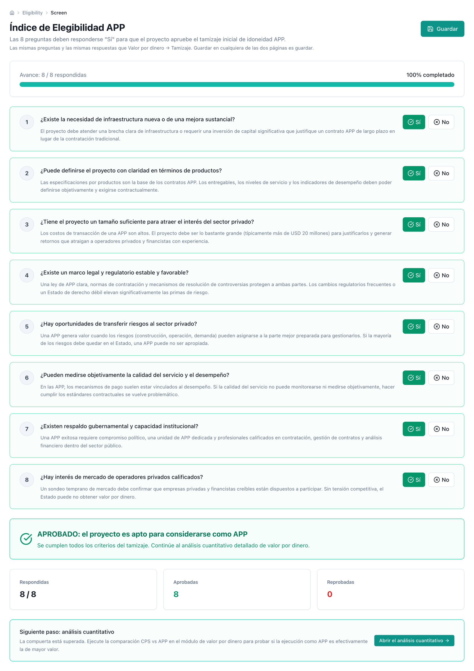
Figure 5.2 — PPP Eligibility Index with the hospital case: the eight questions answered, verdict Passed (8 of 8, none failed) and the next step towards the quantitative analysis.

Step 2 — Complementary qualitative scoring

Labels: PPP Incentive Assessment (Incentives), Qualitative Questionnaire (Questionnaire) and Non‑Financial Benefits. Input: eight incentive factors rated 1 to 4; twenty‑eight yes/no questions in six sections; ten non‑financial‑benefit criteria in three categories, on four levels, with a selectable sector that unfolds its guidance. Output: score, percentage and level on all three —incentives out of 32, questionnaire out of 28, benefits out of 40, with the thresholds published in section 3—, and a subtotal per section or category; the questionnaire passes each section with 60 % of "yes". Analyst's decision: every rating is their judgement; the tool infers none from the financial data. Limit: none of the three scores enters the arithmetic of the Public Sector Comparator (PSC) or of the PPP cost: converted into points by the bands of step 2, they feed the qualitative axis of the report's decision map.

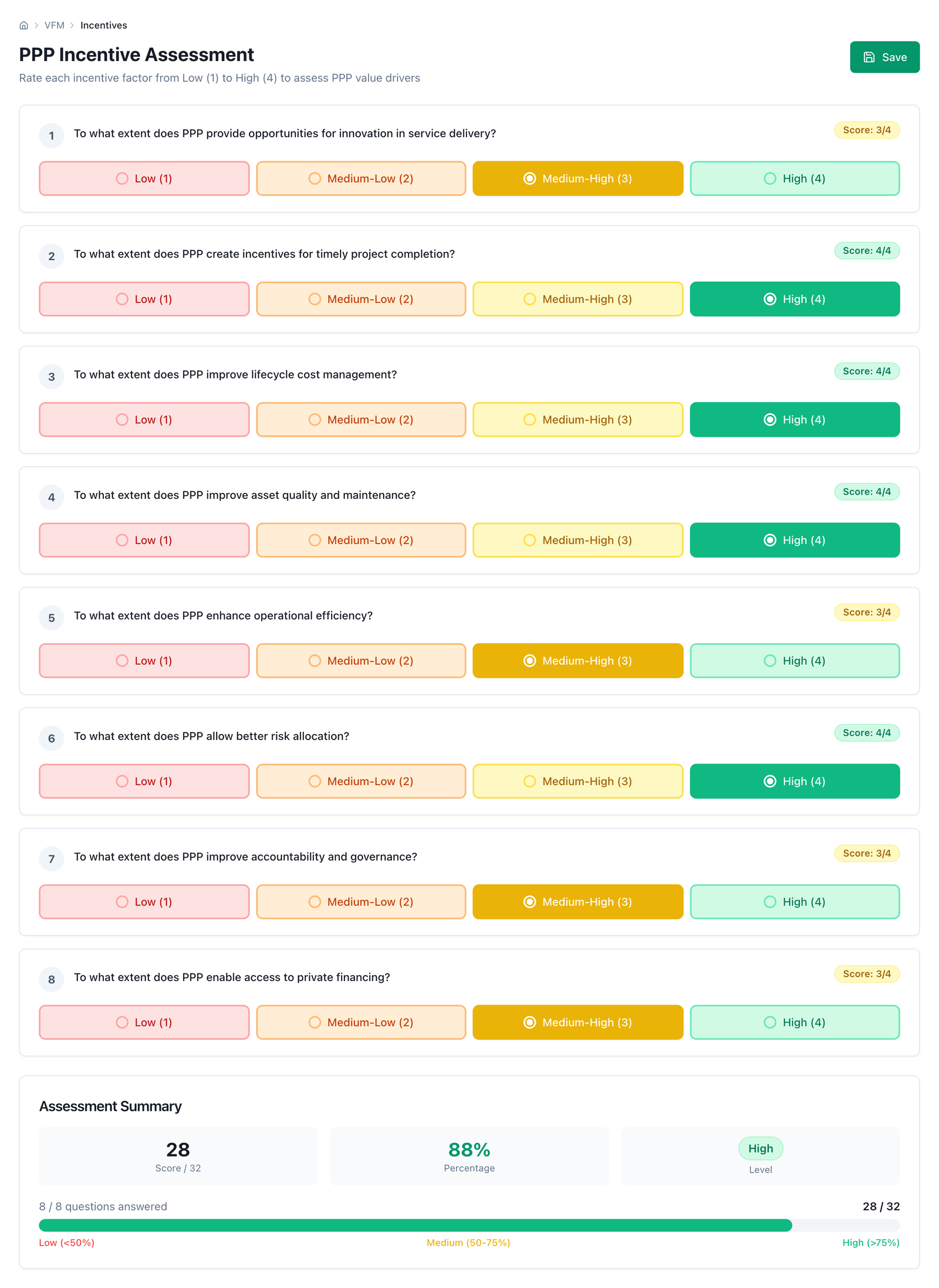
Figure 5.3 — Incentives: the eight factors rated 1 to 4 give 28 out of 32 (88 %, level High), over the 50 % and 75 % threshold legend.

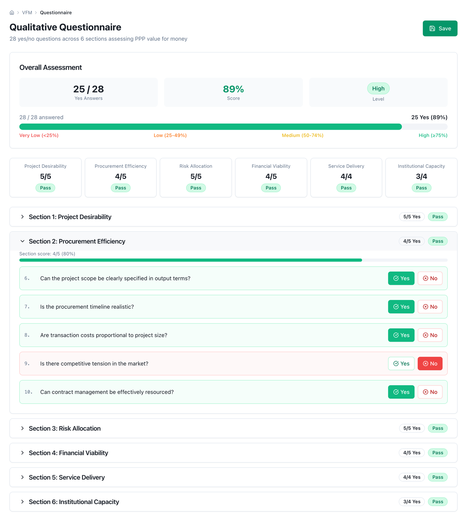
Figure 5.4 — Questionnaire: 25 of 28 "yes" (89 %, level High) and the status of the six sections; the procurement‑efficiency section unfolded, where the only "no" —competitive tension— sits.

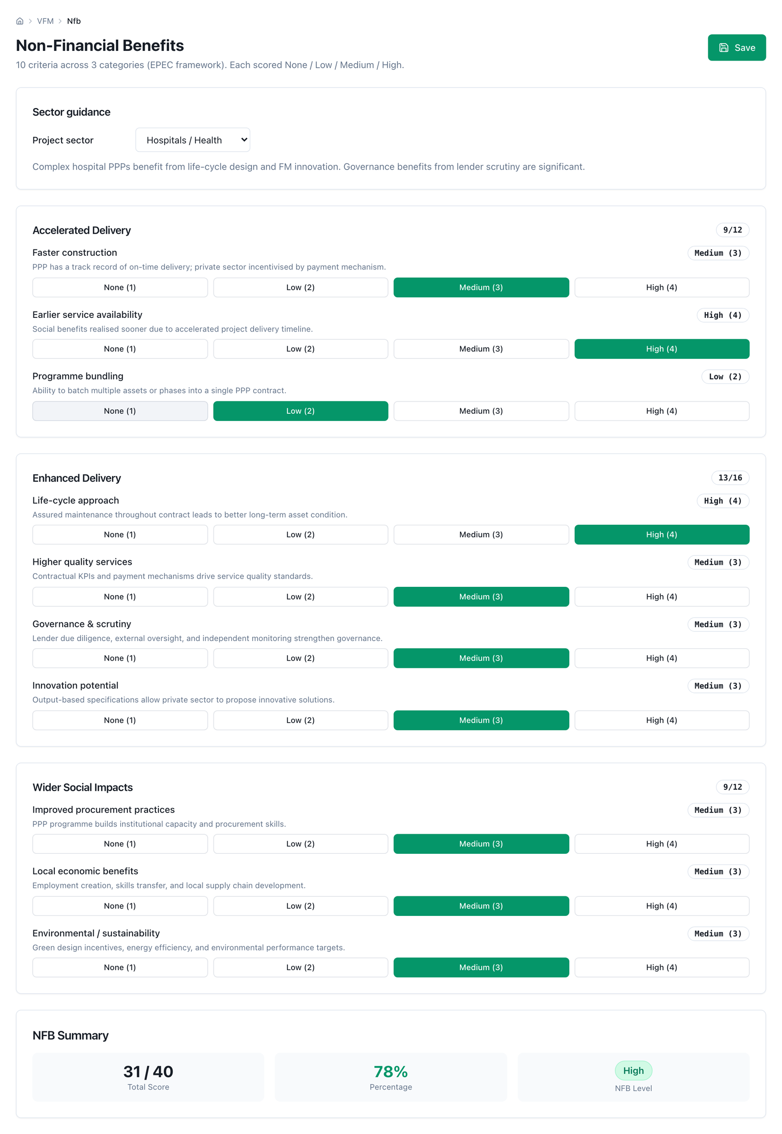
Figure 5.5 — Non‑financial benefits with the hospital‑sector guidance: 9/12, 13/16 and 9/12 per category, 31 out of 40 (78 %, level High).

Step 3 — The project inputs

Label: VFM Project Inputs. Input: the four tabs of step 3 of the method — General and construction (start year, construction period, total investment and by component, schedule, taxes, depreciation and currencies); Operation and maintenance costs (each line with its escalator, maintenance as a percentage of investment and major maintenance with amount and frequency); Revenue (user‑pays, availability or mixed mode, with demand categories, ramp‑up, minimum revenue guarantee and sharing, or the availability payment with its indexation and its window of years); and Financing (tenor, government grant, structure, debt tranches and covenants). Output: the saved scenario, which is the object every other screen reads. Analyst's decision: the whole project model. Limit: the button saves and runs the model at once, and only persists if the engine accepts the inputs —"saved" also means "computable"—; the construction schedule must add up to 1 and the screen flags it if not; and the discount rate, the risk register and the affordability ceiling are not edited here but on their own screens: saving the inputs does not overwrite them.

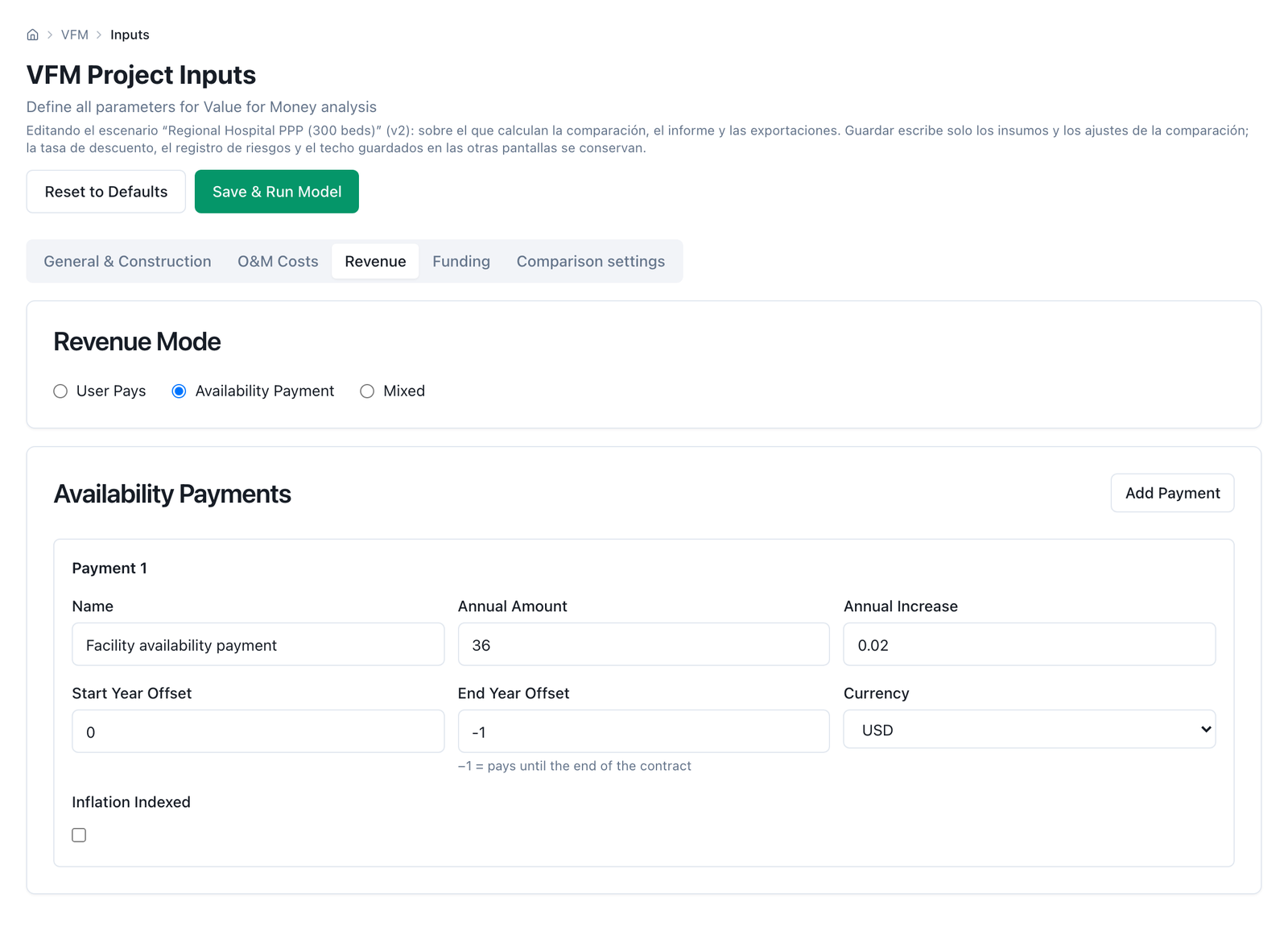
Figure 5.6 — Project inputs, revenue tab in availability mode: a payment of 36 a year indexed at 2 %, from the first operating year to the end of the contract.

Steps 4, 6, 7, 8 and 9 — The PSC vs PPP comparison

Label: Quantitative VfM Analysis. Input: the saved scenario; it asks for nothing else on screen. Output: a validation strip with the input errors and warnings —an empty scenario or one that does not compute is an error with a message, never a number—; the discount‑rate card, which declares which convention ran —a single rate for both legs, or two rates: risk‑free rate plus spread per leg— and where each figure came from: the request, the scenario, the workspace's financial model, or the platform default, the last in yellow and with a warning; on the same card, a label with the risk model that valued the premium —expected value (probability × impact) with its cap, or the legacy optimism bias—; four figures (PSC NPV, PPP NPV, VfM in money and in percentage); and two charts. The rate card is also where the rate is set, in two blocks. The first is the scenario rate for the single‑rate convention: a selector with the library of twelve cited rates with their source —Chile 5.5 %, Peru 8 %, Colombia 9 %, Mexico 10 %, Green Book 3.5 %, World Bank 6 %, European Commission 5 %, among others— prefills it with its citation, the field can be edited, and on saving the rate and its reference stay in the scenario. The second is the rate convention of step 8: a single rate / two rates toggle and, under the second, three fields with their provenance: the government risk‑free rate, with free‑text sourcing (instrument, tenor, basis, date); the PSC spread, with the preset PSC at risk‑free (0 %) or the inverted toll pair (3.3 %); and the PPP spread, with the cited bands from the Australian guidance as presets —none 0 %, low 0.9 %, medium 1.8 %, high 4.8 %— each with its CAPM reading and its footnote citation, or a typed value with its source. The card prints the two resulting rates (PSC rate = 2.70 % · PPP rate = 3.60 % in the hospital), states the rule against double counting and reminds that the cost of capital is not the comparison rate; on saving, the three figures and their sources stay in the scenario and every screen, the simulation and the exports recalculate with them; clearing the risk‑free rate reverts the scenario to a single rate. Below, a table of alternative references recomputes the four figures at the scenario rate, at the Green Book's and at the World Bank's, as a sensitivity. The same card declares how many risks of the register were valued at the neutral values for lack of scoring ("0 of 10" in the hospital), which is the count the reviewer of §3.14 must ask for. Analyst's decision: the convention, the three rate figures with their justification, and the risk model. Limit: the alternative‑references table is a single‑rate sensitivity —it recomputes with the Green Book and the World Bank in both legs even when the scenario runs at two rates— so it reads as the compared reading of step 8, not as a sensitivity to the risk‑free rate (that one is run by changing the risk‑free rate on the card, or on the sensitivity screen); the chart groups the PSC premium in a single bar —the retained‑risk bar on the public side reads zero, because retained risk is reported on the PPP side— and the residual value has no bar of its own; the full breakdown is in the report and the Excel workbook.

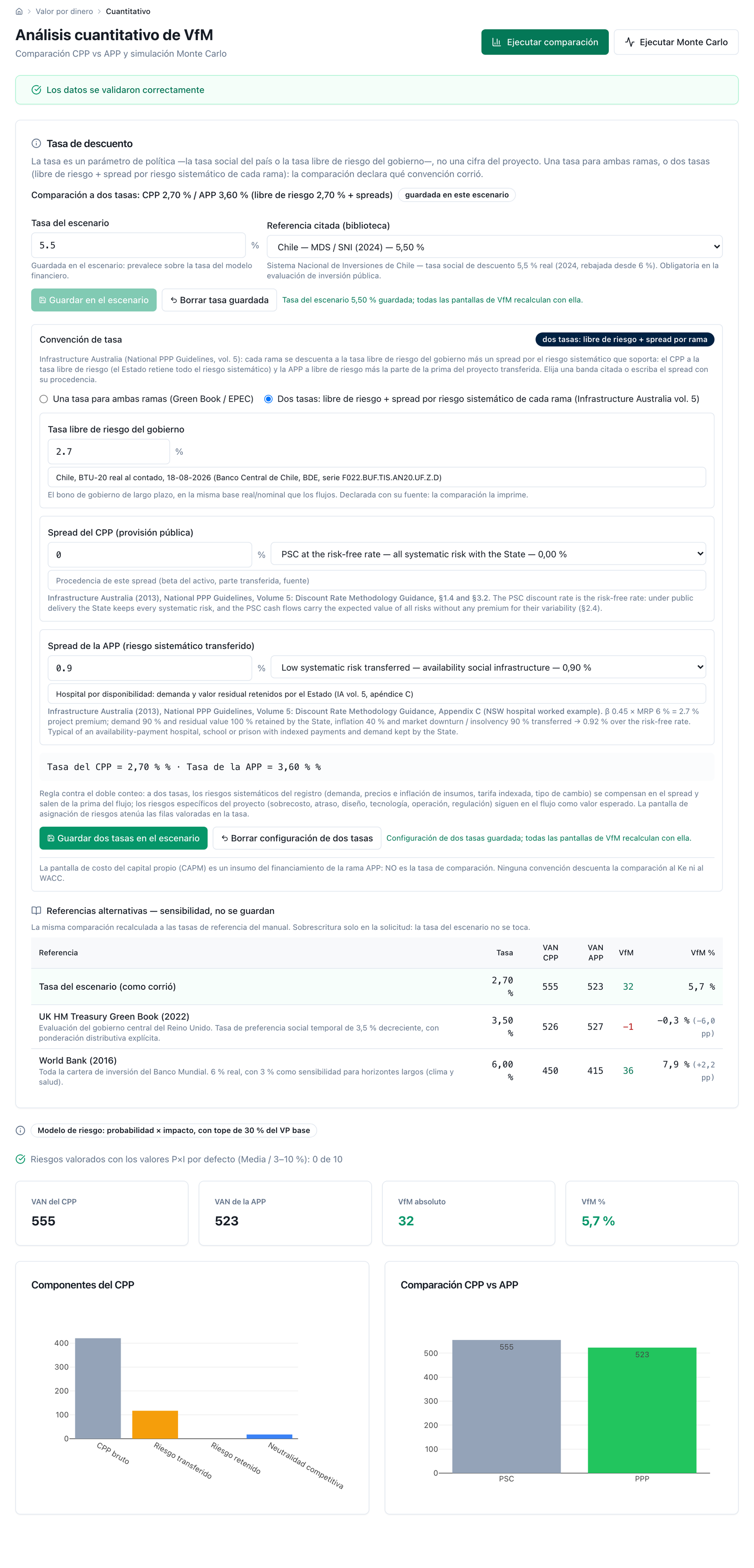
Figure 5.7 — Quantitative analysis at two rates: risk‑free rate 2.70 % with its source and date (BTU‑20 spot, 18‑08‑2026), PSC spread 0 % (preset "PSC at the risk-free rate", the library label is still in English) and PPP spread 0.90 % (low band, appendix C), resulting rates PSC 2.70 % · PPP 3.60 %, expected‑value model with a 30 % cap and "0 of 10" risks scored at the defaults, and the result 555 / 523 / 33 / 5.9 %; below, the single‑rate table of alternative references (Green Book 3.50 % → 526 / 526 / −1 / −0.1 %; World Bank 6.00 % → 450 / 414 / 36 / 8.1 %). The screen rounds the first three figures to whole numbers; the engine gives 555.1 · 522.5 · 32.6. The screenshot predates it and still shows 555 / 523 / 32 / 5.7 % and, in the reference table, 526 / 527 / −1 / −0.3 % and 450 / 415 / 36 / 7.9 %.

Step 11 — Monte Carlo

Label: the Run Monte Carlo button, on the same screen. Input: the scenario and its risk register; the number of runs and the seed have default values (a thousand runs, fixed seed) and can be set programmatically. Output: the label of the risk model under which the draws were taken —the same one the comparison above is valued with—, the probability that the PPP turns out cheaper, the mean, the 5th and 95th percentiles, the histogram with the zero line and a reproducibility row: seed, number of runs and 95 % confidence interval of the mean, which is the stable‑sign diagnostic of step 11. The service response adds the standard error, the runs that would be needed for a given precision and the share of runs in which the premium cap was active. Analyst's decision: how many runs, with which seed, and whether the sign is stable enough to quote. Limit: the simulation does not recompute on its own when inputs change —it is the module's expensive run—: a notice with a button to repeat it appears. The share of capped runs is read in the Excel workbook and in the service response, not on screen.

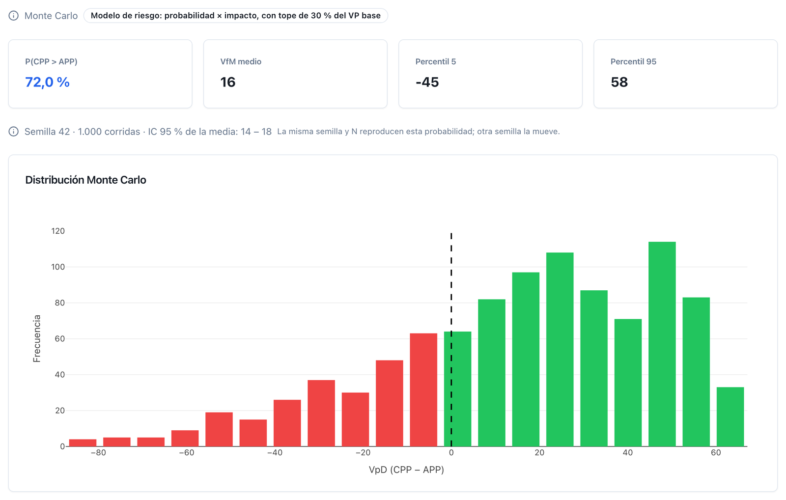
Figure 5.8 — Monte Carlo under the same risk model and the same two‑rate convention: the PPP turns out cheaper in 72.5 % of the thousand runs, mean 17, band −44 to 58, with the seed and confidence interval (15–19) that allow the figure to be repeated. With construction interest computed at mid-year and pro rata, the engine gives mean 16.7, P5 −44.0, P95 58.3 and a 14.7 – 18.6 interval: the screenshot predates it and still shows 72.1 % and mean 16.

Step 10 — Sensitivity and switching values

Label: Sensitivity Analysis. Input: the scenario. Output: a seven‑variable tornado at two rates —investment, operating costs, revenues or demand, the risk‑free rate (which moves both legs at once), the PSC spread and the PPP spread (each only its own leg) and risk parameters—, with the risk‑model label, a chip with the rate convention (two rates: PSC 2.70 % / PPP 3.60 %) and the base VfM; at a single rate the three rate bars merge into one and there are five variables. And a table with the base value of each variable, the VfM at −10 % and at +10 %, the range and the switching value: the change that wipes out the VfM. When a variable has no switching value —the PSC spread, which is zero— the cell says so instead of inventing one. Analyst's decision: reading whether the verdict is fragile; a switching value smaller than the input's estimation error is fragile, whatever the central point says. Limit: the range is fixed at ±10 %, which for a risk‑free rate of 2.70 % is 27 basis points: the risk‑free rate's range sensitivity (§4.4a) is run by changing it on the rate card, not here.

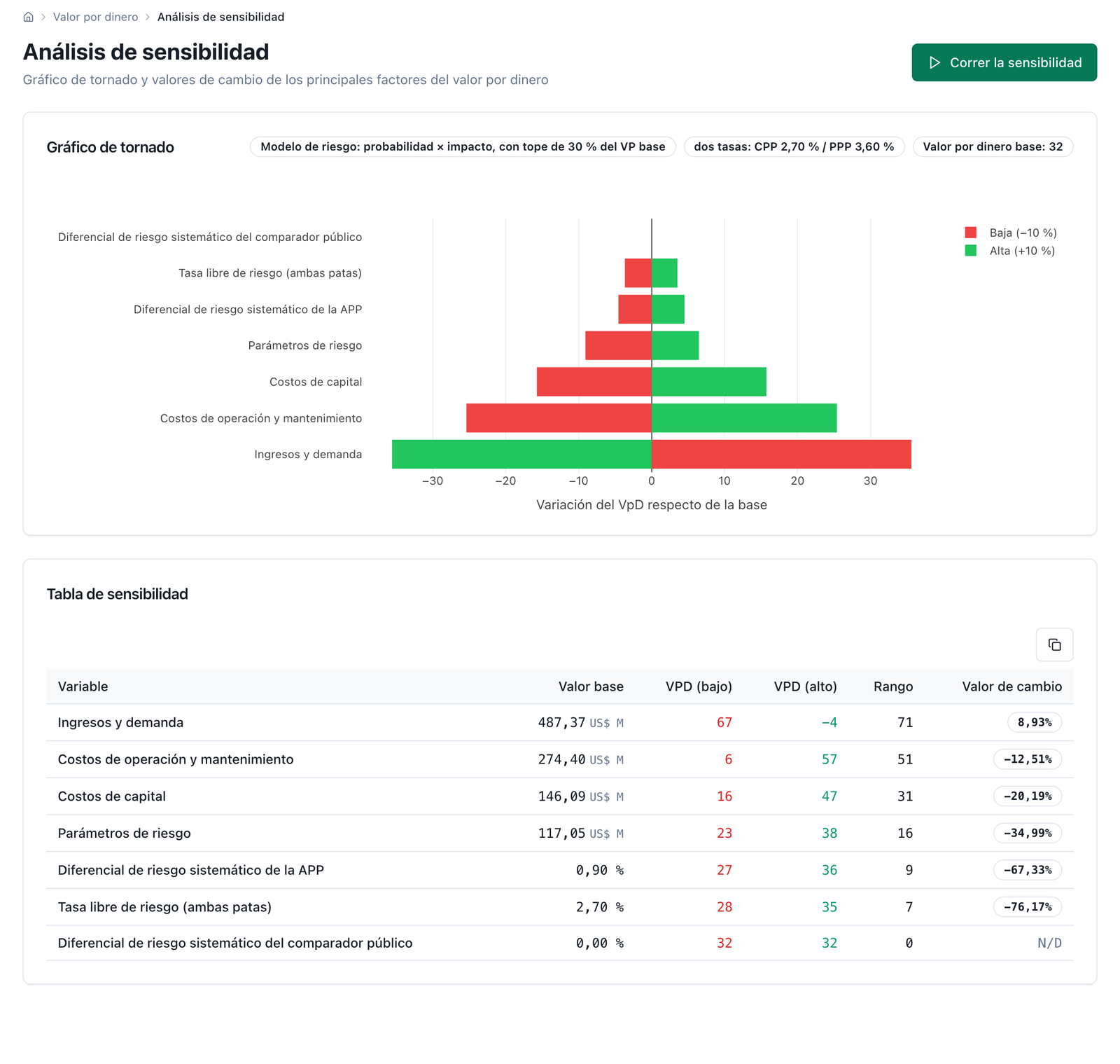
Figure 5.9 — Sensitivity at two rates: the seven‑variable tornado over a base VfM of 33 (32.56 in the engine) —the risk‑free rate moves both legs, each spread moves its own, the PSC spread is a flat bar with no switching value, "N/D" on screen (the Spanish abbreviation)— and the switching values: the payment wipes out the VfM when it rises 9.16 %, operating cost when it falls 12.82 %, capital cost when it falls 20.59 %, the risk parameters when they fall 35.86 %, the PPP spread when it falls 69.04 % (to 0.28 %), the risk‑free rate when it falls 78.17 % (to 0.59 %). The screenshot predates it and still shows a base VfM of 32 and switching values of 8.93 / 12.51 / 20.19 / 34.99 / 67.33 / 76.17 %.

Step 8, note — Cost of capital

Label: Cost of Equity & WACC. Input: a reference sector —eleven profiles with their typical beta and gearing, editable—, risk‑free rate, market return, unlevered beta, country premium and size premium; and, for the structure, pre‑tax cost of debt, tax rate and gearing. Output: cost of equity, after‑tax cost of debt, WACC and the breakdown that adds up line by line to both. Analyst's decision: the premia and the structure; the sector profiles are a starting point, not project data. Limit —and it is the reason for capturing this screen—: the WACC is not the comparison rate, and the screen says so on its first line: the Ke and the WACC are inputs to the financing of the PPP leg; the PSC and the PPP are discounted at the convention set on the quantitative screen —a single social rate on both legs, or the government's risk‑free rate plus a spread per leg. That the tool now admits two rates does not change this: the second rate is the risk‑free rate plus the spread for the systematic risk transferred (3.60 % in the hospital), not the partner's WACC (7.06 %) or its Ke (13.63 %), which also remunerate the project‑specific risk already in the payment; discounting the PPP at the WACC and the PSC at the social rate still manufactures value for money out of nothing. A calibration detail: the engine also adds an illiquidity premium, 1 % by default, which the screen exposes as one more line of the breakdown and which the analyst can set to zero; the figure shown after Calculate is the engine's, and Save to scenario stores it so the report and the Excel workbook print it.

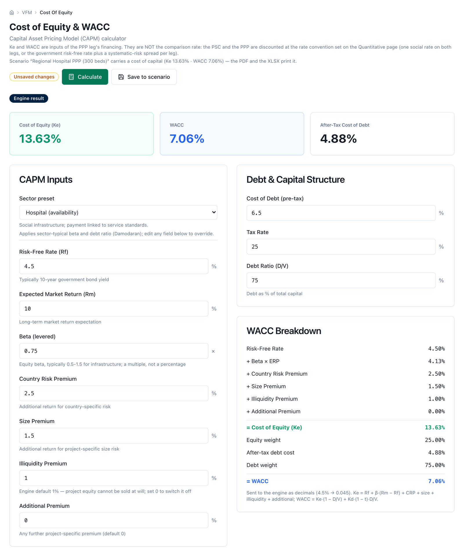
Figure 5.10 — Cost of capital with the availability‑hospital profile: Ke 13.63 % and WACC 7.06 %, computed by the engine and broken down line by line, illiquidity premium included. The header note says so: neither is the comparison rate, under either convention.

Step 5 — Risk register and allocation

Label: Risk Allocation. Input: a type of works that loads a reference table of optimism‑bias uplifts; four blocks of risks —construction, operation and maintenance, demand and renegotiation— with their uplift, their deviation, their allocation on five grades (from fully retained to fully transferred) and a box to include them in the simulation; and a register where every risk receives probability, impact (five bands of percentage of base cost), phase, nature and mitigation. The Nature column offers automatic —the classification by type and phase from step 5, which the screen shows in parentheses: specific or systematic— and the two explicit options to correct it risk by risk. Output: a probability × impact heat map with every risk placed, and a preview of the expected premium —each risk's contribution and the total— with a cap notice; at two rates, the rows for systematic risks appear dimmed, with the caption "valued in the rate", and a footer states how many there are and what the gross premium would be if every risk entered the flow (in the hospital, one row, and the same premium, because its base is zero). Analyst's decision: the scales are published, but the rating of each risk, its nature, its allocation and the choice of model are theirs, and what they edit is saved in the scenario's register, with a version: it is the register the comparison, the simulation and the exports read. Limit: the preview is priced by the same engine that runs the comparison —in the hospital at two rates, gross premium 124.6 against a ceiling of 134.3: the cap does not bind— and is recomputed on every edit of the register without saving it; the figure that rules is still the one on the quantitative screen and in the report. The uplift table by type of works and by risk is Austral's own disaggregation; the British source publishes uplifts by type of works.

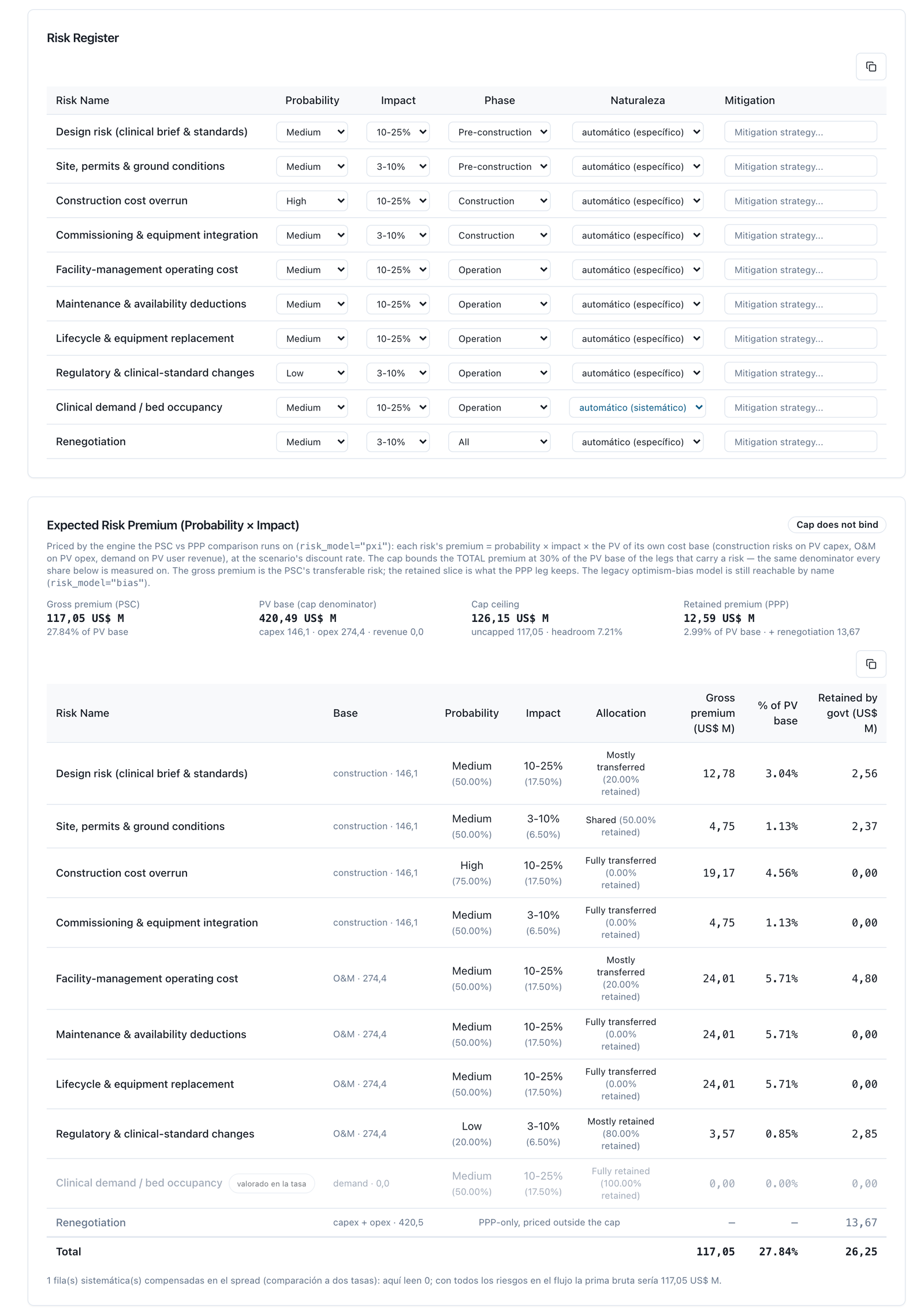
Figure 5.11 — Risk allocation at two rates: the ten‑risk register with the nature column (nine specific, clinical demand systematic) and the preview of the expected premium as priced by the engine —117.05 against a ceiling of 126.15, "the cap does not bind"—, with the demand row dimmed as "valued in the rate". The probability × impact heat map, which sits between the two blocks on screen, is omitted from the figure.

Step 12 — Affordability

Label: Affordability Assessment. Input: two figures the analyst types —the annual budget ceiling for PPP payments and, optionally, GDP— and the profile of government payments the tool derives from the scenario. Output: the maximum annual payment and its percentage of the ceiling, with a traffic light at the 5 % and 10 % bands; the total commitment and its percentage of the term's budget capacity; the present value of the commitment and, if GDP was given, its percentage; and the annual profile charted against the ceiling line. Analyst's decision: the ceiling and GDP, which are fiscal‑policy data and do not come out of the model; both are saved with the scenario, the screen prefills them on return and the PDF report and the Excel workbook print the full block with the annual profile. Limit: a positive VfM does not make a project affordable: firm commitments and contingent liabilities are the subject of manual M2.

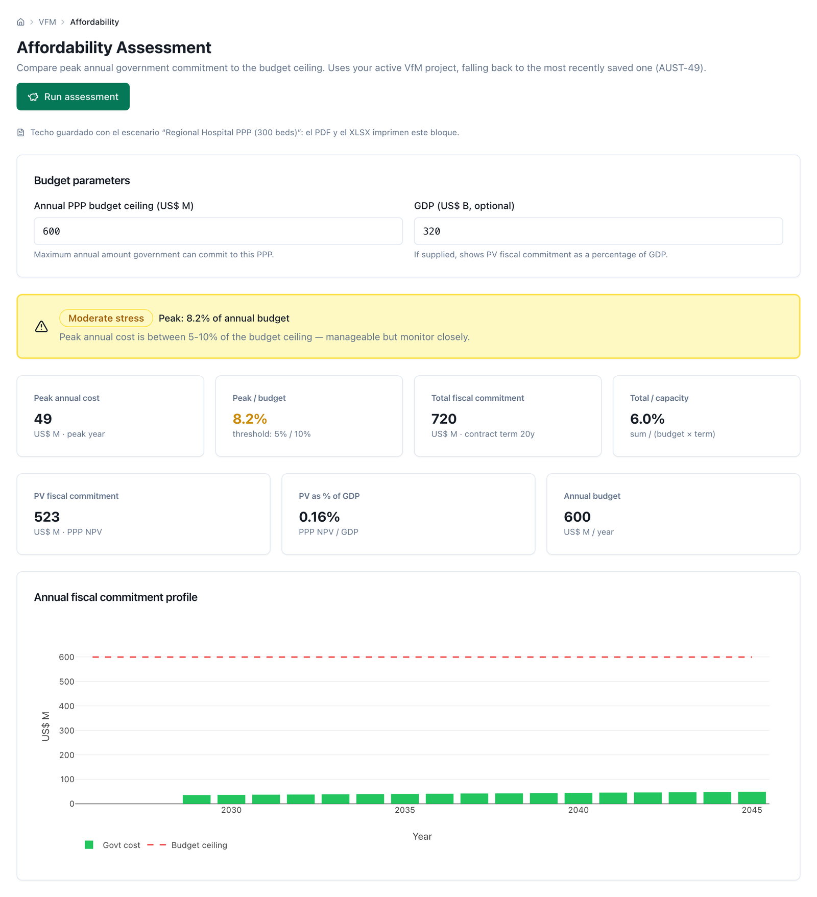
Figure 5.12 — Affordability with a ceiling of 600 and a GDP of 320: the maximum payment of 49.4 is 8.2 % of the ceiling —a moderate reading—, the present value of the commitment is 523 at the PPP‑leg rate, and the annual profile runs well below the line.

Step 9 — Report and combined verdict

Label: VfM Report. Output: a combined‑verdict banner —positive, marginal, conflicting, negative, incomplete or not interpretable— with its headline and a paragraph that explains it, which the screen prints today under the label "screening signal" and below the decision map, which heads the banner; the decision map of six qualitative levels by five probability bands of step 9, calculated on the same qualitative answers and the same simulation, with the scenario's cell framed, its verdict and its reading sentence, and the list of missing instruments if the axis is incomplete; the qualitative and quantitative summaries; and the download buttons. Two behaviours that are worth showing in the capture: a positive VfM with a failed filter is labelled conflicting, not positive; and when the PSC is not a positive present value, the percentage is suppressed —not printed— and the verdict becomes not interpretable, with the instruction to read the VfM in money and review the rate. Analyst's decision: the reading; the verdict is a band, not an investment recommendation. Limit: the banner carries two readings that look at different evidence and may disagree —the screening signal is the qualitative gate plus the point VfM; the map is the four qualitative instruments plus the Monte Carlo distribution— and the screen itself breaks the tie: decide by the map; the signal is the screening reading. Without a simulation the map has no column and says so.

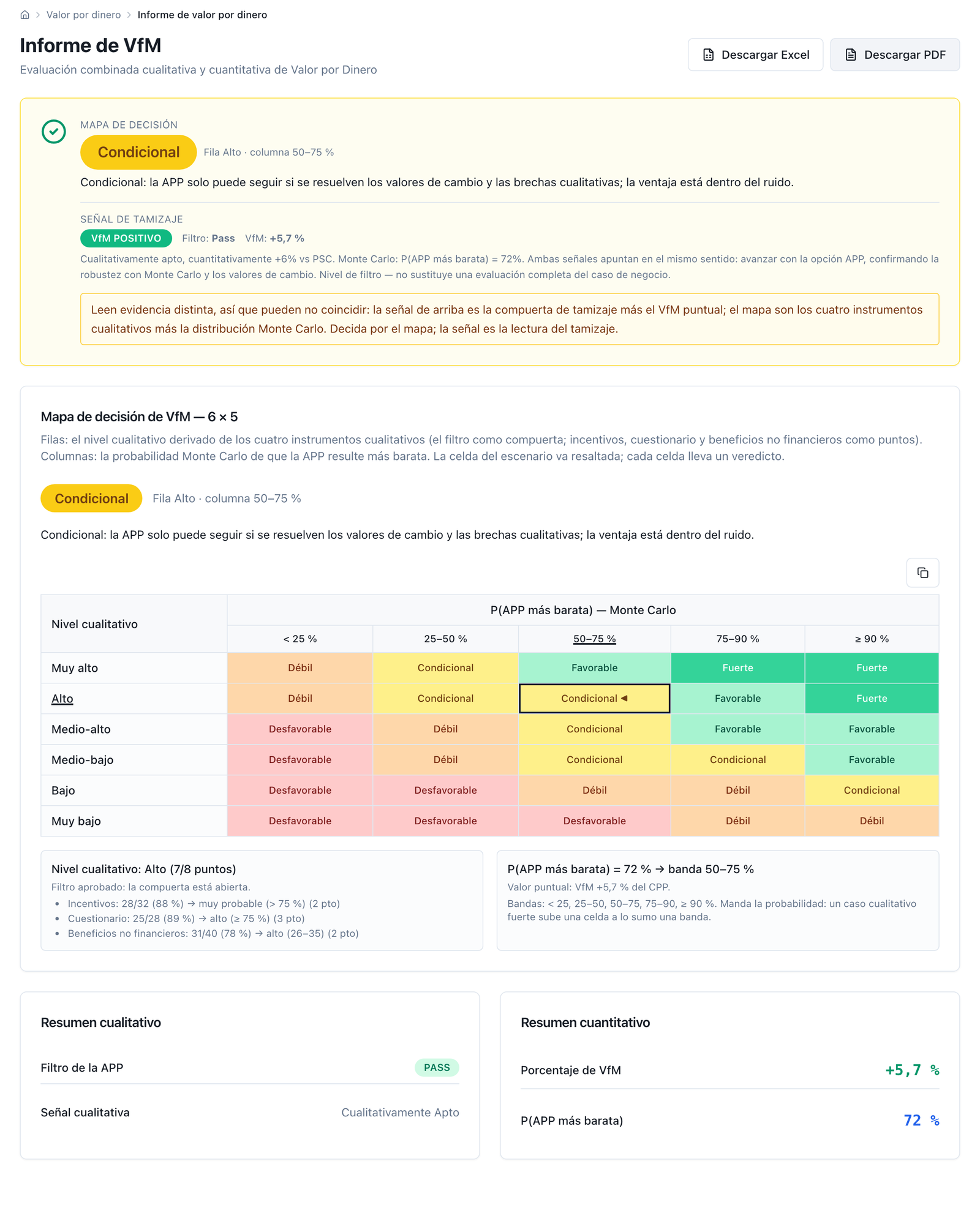
Figure 5.13 — Report at two rates. The banner no longer gives a single verdict: it is headed by the DECISION MAP — Conditional (row High · column 50–75 %), "the PPP can only proceed if the switching values and the qualitative gaps are resolved; the advantage is inside the noise"; below it comes the SCREENING SIGNAL — POSITIVE VfM, filter Pass, VfM +5.9 % ("qualitatively fit, quantitatively +6% vs PSC. Monte Carlo: P(PPP cheaper) = 72%" —the report prints "+6% vs PSC" in English—); and it closes with the box that says why the two can diverge: "they read different evidence… decide by the map; the signal is the screening reading". Further down, the map of six levels by five bands with the scenario's cell —High (7/8 points) × 50–75 %— framed, and the two summaries: +5.9 % and P 73 %. The screenshot predates it and still shows +5.7 % and P 72 %.

5.3 The hospital example, run on the platform

The hospital demonstration pack is the example of section 4: 300 beds, US$ 150 M of investment (design 8, land 7, works and base equipment 120, other 15), three years of construction (30/40/30 %), a 20‑year contract, operating costs of the order of US$ 17.7 M in the first year plus periodic equipment replacement, an availability payment of US$ 36.0 M a year indexed at 2 %, no government grant, 80/20 financing and a ten‑risk register with the allocation of an availability contract: design, construction, maintenance and replacement with the private party; clinical demand and regulatory change with the State. All figures are generic.

With competitive neutrality at 12 % of the present value of the investment, oversight at 2 % a year, no residual value or transaction cost and under the expected‑value model, the result under the two rate conventions is:

Figures in US$ M of present value. At two rates the PSC breaks down into 420.5 of raw PSC, 17.5 of competitive neutrality and 117.1 of risk premium —the nine project‑specific risks; the systematic risk goes into the rate; the 30 % cap is not active: the ceiling would be 126.2— and the PPP cost into 496.3 of government payments net of taxes, 12.6 of retained risk and 13.7 of renegotiation risk. The PSC is positive on every row, so the percentage can be read; at two rates the sign only turns with a risk‑free rate of 0.59 % or a spread of 0.28 %, and at a single rate between 3.5 % and 5.5 %. Under the legacy optimism‑bias model, uncapped, the base case would give +17.1 %: a difference the report makes visible by naming the model.

Reproduce it in four steps. (1) On the home screen, in the workspace‑data card, choose the hospital pack and load it. (2) Open the quantitative analysis: the comparison runs on its own and the rate card will say which convention it applied and where each figure came from; for the base case, choose two rates, type in the risk‑free rate 2.70 with its source and date, leave the PSC spread at 0 and choose the low band (0.90 %) for the PPP, save and then press Monte Carlo. (3) For the comparative reading, switch back to single rate, choose Chile 5.5 % in the library selector and save. (4) Open Affordability, type in an annual ceiling of 600 and a GDP of 320, run the assessment —the maximum payment lands around 8 % of the ceiling, a "moderate" reading— and download the report and the Excel workbook from the report screen.

5.4 What the team takes away

Executive PDF report, in Spanish, English, French or Portuguese: project cover; headline figures table —PSC NPV, PPP NPV, VfM in money and in percentage, the rate for each leg with its provenance, the "Rate convention" row (a single rate on both legs, or two rates: risk‑free rate with its source, each leg's spread with its band and the resulting rate, and the flow premium with and without systematic risks) and the risk model—; simulation results with their reproducibility row (seed, runs, confidence interval of the mean); line‑by‑line breakdown of the two legs with the count of risks valued at default; qualitative block; 6 × 5 decision map with the scenario's cell; affordability block with the annual profile; and a written conclusion. If the PSC is not positive, the percentage cell says it is not interpretable instead of printing the number. There is no filler report: on an empty workspace or a scenario that does not compute, the download is refused with a message. It also carries the tornado —base value of each variable, VfM at ±10 %, range and switching value— and, when the scenario stores a cost of capital, the Ke and WACC in the headline with their breakdown.

Twelve‑sheet Excel workbook: summary; screening; incentives; questionnaire; non‑financial benefits; PSC vs PPP; Monte Carlo; sensitivity; switching values; decision map; affordability; and risk allocation. The summary and the comparison sheet print the rate convention, the three figures with their provenance, the rate of each leg, the flow premium with and without systematic risks and the risk model; the Monte Carlo sheet, the seed, the runs, the confidence interval and the share of capped runs; a section not completed appears labelled as such, not as zero.

Session export and import. The whole workspace —scenarios, with their PSC adjustments and their rate, plus the four qualitative sections— downloads as a single file and loads again into another workspace, replacing what is there or adding to it; the import reports how many scenarios and sections came in and which were skipped, with the reason. It is the way for a reviewer to receive exactly the case they are shown.

Programmatic and batch access. The same computation is available through the API, with the same two rate conventions —the risk‑free rate and the spreads can be declared on each call— and the same declaration of provenance, and there is a batch access —up to one hundred projects per call— to run a portfolio with the same convention, the same base register and the same number of runs.

Assisted analysis. The module's artificial‑intelligence screen generates, over the workspace data, an executive summary, a risk assessment and recommendations. It is a reading aid: the numbers still come from the engine.

And the sentence that matters when closing an engagement: the client keeps the tool and the capacity to operate it. The workspace, the scenarios, the exports and this manual stay in their hands; the work does not end in a report nobody can run again.

5.5 What the tool does not decide for the analyst

The tool computes, declares its assumptions and refuses to print a number that cannot be read. It does not decide the rate convention or its figures: the risk‑free rate, the spreads —from a cited band or typed in— or the single rate are chosen on the card of the quantitative screen and saved with the scenario together with their source; a programmatic call may declare others, a scenario without a rate inherits the workspace financial model's, and failing all of that the screen shows the default with a warning. Nor does it decide the rating of the risk register, its nature or its allocation, competitive neutrality, the residual value, the budget ceiling nor, above all, the reading: a positive VfM with a failed screen is conflicting; a non‑positive PSC obliges a review of the rate before celebrating a percentage; a switching value smaller than the input's estimation error is a fragile verdict.

Two capabilities this manual only names. The risk‑allocation diagnostic against the retention frontier —which transfers create value and which destroy it, in the terms of §2.6— is available as an API call and has no screen of its own. And the module includes an ESA 2010 / Eurostat classifier for on‑ or off‑balance‑sheet treatment, which itself warns that it is a simplified extract of the rules and no substitute for an official ruling, and an asset‑recycling block (valuation of existing assets, lease‑operate‑transfer structure and redeployment multiplier): extensions outside the PSC method, referred to their own documentation.

6. Why not in Excel, for this method

The method of section 3 can be run in a spreadsheet. It is written for that, and the Public Sector Comparator (PSC) of most ministries was and is built in one. This section does not repeat the general argument against the spreadsheet —speed, size, charts, brittle formulas— which holds for any computation and which Austral publishes elsewhere. It is about something else: the five points of the PSC method at which the spreadsheet fails in a way nobody sees, because the number that comes out still looks like a number.

Every failure is presented the same way: at which step of section 3 it happens; a concrete example, reproducible with the hospital of section 4 or with the toll‑road demo; and what the tool does instead, with the screen or the output of section 5 that shows it. The hospital examples are engine runs on the demonstration pack, under the expected‑value model with a 30 % cap and at a single real rate of 5.5 % —the comparative reading of section 4, which was the base case for edition 1.0— unless stated otherwise: the failures this section illustrates do not depend on the rate convention, and the single‑rate reading is the one most PSC spreadsheets recognise; where the two‑rate convention changes the lesson, it is noted. The annex at the end lists every figure with its origin. Several of the episodes that illustrate the failures happened to the tool itself before being fixed. They are told as they were, because they are the section's best argument: it is not that the spreadsheet has errors and the program does not; it is that the program leaves a trace and is fixed once for every case, and the spreadsheet is not.

6.1 Versions of the PSC: the same project, three spreadsheets — which one did the committee approve?

Where it happens. Steps 6, 7 and 8, which is where the PSC adjustments live (risk premium, competitive neutrality, residual value), the PPP‑leg charges (oversight, transaction, retained risk) and the rate; and step 13, when the ex ante PSC has to reappear, intact, next to the bid.

What fails in the spreadsheet. A PSC lives for months. In that time it gets copied: one version for the committee, another "adjusted after the meeting", another the financial adviser returned with the updated model, another for the report. Each copy is opened, a cell is touched and it is saved under the same name. None knows the others exist. When the question is "which version did the committee approve?", the answer is a file with a date, and nobody can say which adjustment that copy lost relative to the previous one.

The damage is not theoretical. On the hospital of section 4, five copies of the same PSC, each with a single adjustment lost, give this:

US$ M in present value. Five files, five verdicts between +2.9 % and +20.3 %, and none "looks wrong": all five spreadsheets are internally consistent, add up and have the same name. Copy B is marginal under the bands of step 9; A is positive; C and D cross the 15 % threshold that opens the strong band. A committee may have approved any of the five.

It happened to the tool. In an earlier version, the on‑screen comparison, the report export and the request default resolved the rate in three different places of the program, with three different pairs of rates, and the downloadable report did not match the screen for the same scenario. Later, on a client case, three surfaces of the same module —the comparison, the report and the verdict— gave three different VfMs because each loaded the saved scenario with its own loader and each loader lost a different adjustment (that case's figures are the client's and are not reproduced here; the pattern is exactly that of the table). The cause was structural —N copies of the logic "load the scenario and call the engine"— and so was the fix: one scenario object and one loader.

What the tool does. The scenario is one object, not a file: the three data blocks (model inputs, model results, risk register) and the six PSC adjustments (rate, competitive neutrality, residual value of each leg, transaction cost, risk model and its cap) are saved together, with a version number that rises on every write; two people editing at once do not tread on each other: the second write over a stale version is rejected. Every screen and every export reads that scenario and no other copy: the comparison (capture 7), the Monte Carlo (8), the sensitivity (9), the affordability (12), the report (13), the PDF and the Excel workbook. One rule worth knowing because it is the one that closes copy B: an adjustment saved at zero is an adjustment, not a blank —a competitive neutrality declared at 0 does not revert to the 12 % default. And for step 13, the ex ante PSC is not "filed": it stays saved as a scenario with its version, and the bid VfM is another scenario that cites it; the reconciliation between the two is done with the same six pieces, not with two files someone has to line up again. The home screen (capture 1) shows the list of scenarios with their provenance note, which is what the committee should have in front of it instead of a file name.

6.2 Traceability of assumptions: the rate, the cap and the scales buried in cells

Where it happens. Step 8 (the rate) and step 5 (the two qualitative→numerical scales and the premium cap). They are the three assumptions that move the verdict most and the three that in a spreadsheet live in loose cells, often on a helper sheet, without unit, source or date.

The rate. In the spreadsheet the rate is a cell —0.10, 0.055— referenced from a hundred formulas. The cell does not say where it came from (the country's social rate? the adviser's WACC? the value the template shipped with?), nor who changed it, nor when. On the hospital, the difference between "the template's 10 % stayed" and "the regulator's 5.5 % was entered" is the one separating copy C from the approved one in the table above: +20.3 % against +6.5 %. Both are readings of the same project; only one is the rate that rules. In the tool's history, the warning that today accompanies the default rate was born from a measurement on the toll‑road demo: the same case read +39.2 % with the default rate and −17.5 % with the project's rate —"an inverted recommendation, not a rounding difference", the warning says.

What the tool does. The rate is not a cell: it is a scenario field with provenance. The quantitative screen (capture 7) resolves it in a published order —the one the analyst declares, the one the scenario saved, the one in the workspace's financial model, and only at the end the default— and prints it with its origin: when it comes from the library of cited rates, the label says which country, which body and which year ("Chile — MDS / SNI, 5.50 %"); when it is the default, it is shown in yellow with a warning. The same label travels to the PDF and the Excel workbook. Changing the rate is a write on the scenario, with a version: the question "who changed 10 % to 5.5 %, and when?" has an answer.

Two rates without a rule, one per leg. It is the error step 8 names first, and the spreadsheet commits it effortlessly: it is enough for the PPP leg to be discounted on another sheet, with another cell —"at the bidder's cost of capital", "at the adviser's WACC". That the method uses two rates does not change this: the two rates of step 8 start from the same risk‑free rate and differ only in a spread for systematic risk, with provenance; a pair of rates chosen without that rule is exactly the artefact the step forbids. On the hospital:

The same hospital, the same register, the same neutrality: between −16.7 % and +35.8 % with a pair of rates alone and no rule. Neither of those two figures is a computation error; both are the artefact step 8 forbids. The two rows with a rule —a social rate on both legs, or the risk‑free rate with a cited spread— move between +5.9 % and +6.5 %, and the difference between them is a declared decision, not a cell. In an earlier version of the tool, the comparison itself ran with two different rates on each leg, chosen ad hoc, and the demo's verdict changed sign just by equalising them. What the tool does today: it does not admit two loose rates. The two rates are built on the rate card (capture 7) from a common risk‑free rate with its source and a spread per leg with its cited band or its justification; the old per‑leg rate fields are accepted for compatibility but reduced to the same value; and every call to the engine passes the two resulting rates together with the rule against double counting. The cost‑of‑capital screen (capture 10) exists to say out loud that the WACC is not the comparison rate under either convention.

The premium cap. The 30 % of step 5 is one more cell in the spreadsheet, and one of the least visible: hardly anyone remembers it exists until it bites. On the hospital the expected premium is 97.4 and the ceiling at 30 % is 104.7 —it does not bite. If someone "conservative" lowers it to 20 %, the premium is cut to 69.8 and VfM lands at +0.6 %; at 15 %, −3.6 %; at 10 %, −8.1 %. A cell nobody looks at inverts the verdict. What the tool does: the cap is a scenario adjustment, it is printed next to the name of the risk model on the rate card (capture 7) and in both exports, and the risk screen (capture 11) shows the uncapped premium, the ceiling and whether the engine had to scale down.

The scales. The spreadsheet has a register with "High", "Medium", "10–25 %", and on another sheet —or in the analyst's head— the table that turns each word into a number. Three things happen without anyone seeing them:

• A level changes at a meeting. If the hospital's construction overrun goes from probability "High" to "Medium" —one word, in one cell—, the PSC premium falls from 97.4 to 91.1 and VfM from +6.5 % to +5.2 %. If the equipment‑replacement risk drops from the "10–25 %" band to "3–10 %", VfM lands at +4.1 %, that is, it changes band (marginal). Nobody will notice, because the register still looks reasonable.
• The register is not scored. A register with overrun bands but no probability or impact assigned falls, risk by risk, on the neutral values (0.50 and 3–10 %). On the hospital that is worth a premium of 45.4 instead of 97.4 and a VfM of −5.2 %: a negative verdict that measures not the project but the absence of a risk workshop. It happened to the tool: its flagship demo carried for months a register with bands and no levels, and under the expected‑value model its ten risks were all valued the same; the demo's PSC premium went from 135 to 345 the day it was scored, and the sense of the verdict became explained instead of guessed.
• The scale itself changes. If on the helper sheet the midpoint of "10–25 %" goes from 17.5 % to another value, all ten premiums change at once and no formula "breaks".

What the tool does: the two scales are those of step 5, published and fixed; the scored register is saved in the scenario from the risk screen (capture 11), with probability, band, phase, allocation and mitigation per risk; the premium preview shows each risk's contribution, so a change from "High" to "Medium" is visible as a row going down; and the comparison prints how many risks were valued at default —on the rate card of the quantitative screen (capture 7), in the PDF breakdown and on the risk‑allocation sheet of the workbook—, which is the count the reviewer of §3.14 must ask for; the side‑by‑side comparison of the two risk models, available programmatically, adds what share of the premium they explain.

6.3 Monte Carlo: what an honest simulation costs in a spreadsheet

Where it happens. Step 11, and by rebound step 9, because the probability P(PSC > PPP) is the second requirement of the strong band.

What it costs in the spreadsheet. An honest simulation of step 11 requires, per run and per risk, an occurrence trial with the scale's probability, a uniform draw within the impact band, multiplication by the phase's base, the split between legs by the retained fraction, the cap applied to every run and the run's VfM. A thousand runs by ten risks by two legs: twenty thousand draws and a thousand caps. In Excel that is a macro or an add‑in, and with either of the two there are four things that are almost never done:

1. Seed. Without a fixed seed, two runs of the same case give two results. In the tool's history, two downloads of the same report ninety seconds apart gave US$ 1.0 M of difference in the mean and US$ 6.5 M at the 95th percentile under the same input‑provenance code —the PDF export drew without a seed. On the hospital, three unseeded runs of a thousand draws each give means of 17.0, 17.1 and 18.8 and probabilities of 76.8 %, 76.0 % and 79.0 %; with a fixed seed, two runs give the same result to the last decimal. And it is not cosmetic: with seed 42 the hospital's probability is 77.7 %; with seed 7, 75.3 %: two and a half points on the same case, and both within three points of the 75 % the strong band requires. A verdict that depends on the seed and does not publish it is not a verdict.
2. Correlation. Construction overruns and land delays go together. Drawing them independently is a strong assumption; drawing them correlated in a spreadsheet is a Cholesky decomposition almost no PSC does. The tool also draws them independently —step 11 says so and this section declares it— but it says so, which is the difference.
3. The cap per run. Capping each run and then averaging gives less than capping the average. On the hospital the cap bites in 41 % of the PSC runs, and that is why the simulated mean (17.3) sits below the deterministic VfM (30.0). A spreadsheet that does not apply the cap per run —or applies it and does not say how many times— delivers a mean that cannot be reconciled with the central point, and the reviewer concludes one of the two is wrong.
4. Sampling something else. The gravest failure and the least visible: the simulation samples a different risk model from the one the deterministic comparison next to it uses. An inherited spreadsheet carries the macro written for the uplift model (a truncated normal around a mean bias, uncapped) while the comparison table has already moved to capped expected value. It happened to the tool, and it was fixed: on the toll‑road demo, the comparison said +19.2 and the simulation beside it had a mean of +192 with 100 % probability. On the hospital, today, the simulation under the legacy model would give a mean of 96.5, a probability of 99.9 % and P5–P95 of 48.7 to 144.4; under the model the comparison uses, a mean of 17.3, a probability of 77.7 % and P5–P95 of −30.4 to 51.0. Same register, same hospital: one histogram says "the PPP always wins" and the other says "it wins three times out of four and can lose by 30". Only the second is centred on the comparison the committee has in front of it.

And convergence, which is not computed in a spreadsheet: with 100 runs the hospital's mean is 16.9 and its 95 % confidence interval runs from 11.7 to 22.1; with 1,000, 17.3 and [15.7; 18.9]; with 10,000, 17.5 and [17.0; 18.0]. The sign is stable from 100 runs —the interval never crosses zero—, but the 5th percentile moves from −41.8 to −30.4 between 100 and 1,000 runs. Whoever quotes a P5 at 100 runs quotes noise.

What the tool does. The Monte Carlo button (capture 8) draws the same model as the comparison —Bernoulli by the scale's probability, uniform within the band, cap per run with the same denominator— and labels it so on screen, next to the model's name, so that nobody reads a histogram of one model under a comparison of another. Seed and number of runs are published constants (42 and 1,000), can be changed programmatically and the response returns them with their basis ("explicit" or "default"). The response also carries the convergence block —standard error, confidence interval of the mean, whether the sign is stable and how many runs a given precision would take— and the share of runs in which the cap bit, which is what explains the gap between 17.3 and 30.0 instead of leaving it a mystery. The same reproducibility row —seed, runs, confidence interval of the mean— is drawn on screen (capture 8), printed in the PDF and on the Monte Carlo sheet of the Excel workbook, which adds the share of capped runs.

6.4 Comparison across projects: twenty hospitals, twenty spreadsheets

Where it happens. Steps 8 and 9 (the rate and the verdict have to be comparable) and step 12 (the portfolio is what goes to the fiscal registers of manual M2).

What fails in the spreadsheet. A ministry with twenty hospitals in its pipeline has twenty PSCs, built by three teams over two years, each with its rate, its scale table, its cap and its version of the macro. Ranking them by VfM is copying twenty cells to a new sheet. The order that comes out means nothing, because each VfM is measured with a different ruler —and §6.2 showed how much each ruler moves.

Two projects are enough to see it. The hospital of section 4 and the toll‑road demo, each read "at its own rate": the hospital at the regulator's 5.5 %, the toll road at the 10 % its spreadsheet carried:

The toll road "wins". With the same convention on both (here, a single rate):

At 10 % the order flips; at 5.5 % the toll road is not even comparable, because it is a self‑financing project whose PSC is not a positive net cost (section 3, step 4). A sheet of twenty cells knows none of this: it ranks "+154.9 %" above "+6.5 %" and the hospital comes last.

What the tool does. One engine and one convention for the whole portfolio. The workspace's scenarios run with the same rate convention (the same risk‑free rate, and a per‑project spread drawn from the same table), the same scales, the same cap, the same risk model and the same number of runs, and every result declares those five things in its response, so that two VfMs from the same workspace are comparable by construction. Batch access (§5.4) does the same for up to a hundred projects per call, with the same rate convention and the same declaration of provenance: the portfolio table comes out of one run, not twenty files. And the not interpretable regime is flagged rather than printed, so the toll road appears in the table as what it is —a project read in money that obliges a review of the rate— and not as first in the ranking. What follows onward —firm payments to the commitments register, guarantees to the contingent one— comes out of the same scenarios into the modules of manual M2, not out of a manual compilation.

6.5 Audit: what an auditor can reconstruct three years later

Where it happens. Step 13 (the ex ante PSC must reappear next to the bid), step 9 (the verdict must be reproducible) and the checklist of §3.14.

What fails in the spreadsheet. Three years after the award, an auditor receives a file. They find: a VfM number; a rate in a cell without a source; a register with words and a scale sheet that may not be the one that was used; a Monte Carlo macro that may not run in their version of Excel and, if it runs, gives another result because it has no seed; and no way of knowing whether that file is the copy the committee approved or the one touched up afterwards. Of the eight items the reviewer of §3.14 must ask for, they can verify the first —the number— and none of the other seven.

Two documented episodes of the tool show the other extreme: the spreadsheet that shows a plausible number when there is no data, and the percentage that changes sign without anyone seeing.

• The filler report. In an earlier version, the PDF report download on a workspace with no saved scenario at all returned a complete document, with letterhead, reading "VfM +12.3 %", with a PSC, a PPP and a 72 % probability. They were placeholder constants nobody had computed, and nothing on the page said so. The same happened with a real scenario the engine could not value. Today an empty workspace or a scenario that does not compute produces no document: the download is refused with a message saying what failed, and a guard prevents any result constant from existing in the module again. A spreadsheet cannot promise that: it always shows what is in the cells.
• The percentage with the inverted sign. On the toll‑road demo, at 4 % and under the legacy model, the adjusted PSC is −113.9 and the PPP cost +376.7: the PPP is US$ 490.6 M more expensive. The ratio VfM / PSC gives "+430.9 %", and an earlier version of the tool printed it with the headline "Positive VfM for the PPP". Under the current model the same demo at 4 % gives a PSC of −604.9 and a VfM of −768.6, which the spreadsheet would write "+127.1 %"; and at 8 % a PSC of 19.4 —almost zero— produces a "−756.7 %" that is pure denominator noise. Today any non‑positive PSC flags the verdict as not interpretable, suppresses the percentage and says so in the report (capture 13). The hospital never enters that regime —its PSC is positive at all four rates—, and that is precisely why it was chosen as the main example and the toll road as a box.

What the tool does. What the auditor receives is not a file but a saved scenario with a version, plus the exports that cite it:

To that is added the provenance the exports carry: the PDF prints in its footer the workspace, an input code (the cryptographic digest of the data it was computed with, which changes if any figure changes), the engine version, the deployed program version and the date and time. If the auditor recomputes with the same inputs and gets the same code, they are looking at the same case; if not, they know something changed and can ask what. And the session export (§5.4) packages the whole workspace —scenarios with their adjustments and their rate, plus the four qualitative sections— to load into another workspace: the auditor receives exactly the case, runs it, and gets the same verdict, the same distribution and the same code. It is the audit trail step 13 asks for and that a three‑year‑old .xlsx cannot give.

6.6 Summary: failure → step → what fails in the spreadsheet → what the tool does

6.7 What the spreadsheet does well

It would be dishonest to close without saying it. The spreadsheet is the best tool for prototyping: the hospital of section 4 itself was calibrated by iterating figures until the PPP leg was bankable and the VfM legible, and that iteration is faster in a sheet than on any screen. It is the best tool for explaining a formula: section 3 is written so that every step fits in a column, and a reviewer who wants to understand why the hospital's premium is 97.4 does well to rebuild it in ten rows —probability × band × base— before arguing it. And it is the best tool for teaching: a PSC of three projects on one sheet teaches more than twenty in a portfolio. The Rancagua public comparator (box 4.11) was built in a spreadsheet and is a serious document; most of those cited in section 2 were too.

That is why the tool exports to Excel a twelve‑sheet workbook: so that the spreadsheet remains the place where things are explained and argued. What changes is where things are decided and defended: in a versioned scenario, with the rate and its source, with published scales, with a simulation that samples the same thing as the comparison and with a provenance footer an auditor can verify three years later. And it is worth remembering that the tool did not get there by design: it got there by fixing, one by one, the failures of this section after committing them. That is the real difference from the spreadsheet. Not that it does not fail; that when it fails, it fails once, leaves a trace, and is fixed for every case at once.

Annex — Origin of every figure in this section

All hospital figures are engine runs on the Regional Hospital PPP (300 beds) demonstration pack of the guest workspace (the same one §5.3 documents), through the same route the comparison screen uses: competitive neutrality at 12 % of the present value of investment, oversight at 2 % a year, no residual value or transaction cost, expected‑value model with a 30 % cap, a single 5.5 % real rate except for the row that says otherwise, US$ M of present value. The demo figures are from the Accra‑Tema Motorway PPP (Ghana) pack. The "documented episodes" are from the tool's history and are cited with the figures recorded at the time.

7. References and further reading

All references were consulted between 12 and 14 September 2026; those added or corrected in edition 1.1 (refs. 9, 25 and 42), on 16 September 2026. Unless stated otherwise, each document was read in its official version (PDF downloaded from the publisher's site or official page). ✔A = verified in an Austral paper with a recorded verification, not re‑read for this manual. Where a document was read in a third‑party compilation or through another reference, it is said.

Primary sources of the manual

1. World Bank, Asian Development Bank & Inter‑American Development Bank (2017). Public‑Private Partnerships Reference Guide, Version 3. Washington, D.C.: World Bank Group. Module 3, "PPP Cycle", §3.2 "Appraising Potential PPP Projects" (§3.2.4 "Assessing Value for Money of the PPP", box 3.5; §3.2.5 "Assessing Fiscal Implications"). https://ppp.worldbank.org/public-private-partnership/library/ppp-reference-guide-3-0 (PDF: https://ppp.worldbank.org/sites/default/files/2024-08/PPP%20Reference%20Guide%20Version%203.pdf).
2. HM Treasury (2026). The Green Book: Central Government Guidance on Appraisal. London, February 2026 edition (replaces those of 2003, 2020 and 2022). Chapter 6 (§6.52–6.57 discounting; §6.67–6.71 risk and uncertainty; §6.78–6.84 optimism bias and contingency) and annex A, "Private finance models" (§A.10–A.18). https://www.gov.uk/government/publications/the-green-book-appraisal-and-evaluation-in-central-government (PDF: https://assets.publishing.service.gov.uk/media/698dbcd17da91680ad7f4308/The_Green_Book_2026.pdf).
3. HM Treasury (2013). Supplementary Green Book Guidance: Optimism Bias. London; published on GOV.UK on 21‑04‑2013 from the Mott MacDonald study (2002). Table 1, "Recommended Adjustment Ranges"; §3.3–3.14. https://www.gov.uk/government/publications/green-book-supplementary-guidance-optimism-bias (PDF: https://assets.publishing.service.gov.uk/media/5a74dae740f0b65f61322c72/Optimism_bias.pdf).
4. HM Treasury (2006). Value for Money Assessment Guidance. London, August 2004, updated in November 2006; quantitative tool (Quantitative Assessment User Guide) withdrawn on 5‑12‑2012. Cited through reference 5; not re‑read in its original version.
5. National Audit Office (2013). Review of the VFM Assessment Process for PFI. Briefing for the House of Commons Treasury Select Committee. London, October 2013. Summary §2, §7; §1.6; §3.15–3.16. https://www.nao.org.uk/wp-content/uploads/2014/01/Review-of-VFM-assessment-process-for-PFI1.pdf.
6. International Monetary Fund & World Bank (2019). PPP Fiscal Risk Assessment Model, PFRAM 2.0 — User Manual. Washington, D.C., September 2019. §II.B "What PFRAM 2.0 Cannot Do"; §III.C "Government Support to PPPs"; §III.D "Accounting and Reporting PPPs" and box 2; §III.E "Fiscal Risks Matrix", table 1; annex I. https://www.imf.org/external/np/fad/publicinvestment/pdf/PFRAM2.pdf (the text was verified on a local copy of the same PDF).
7. World Bank (2022). Managing the Fiscal Implications of Public‑Private Partnerships in a Sustainable and Resilient Manner: A Compendium of Good Practices and Lessons Learned from the COVID‑19 Pandemic. Washington, D.C., August 2022, volume I. https://documents.worldbank.org/en/publication/documents-reports/documentdetail/099170003082331955.

PSC guidelines that set the practice

1. Infrastructure Australia (2008). National Public Private Partnership Guidelines, Volume 4: Public Sector Comparator Guidance. Canberra, December 2008 (Commonwealth of Australia reprint, February 2016). §2.3, §3.2–3.7, §4, §5, §6.2–6.6, §7–§9, §10.4. https://www.infrastructure.gov.au/sites/default/files/migrated/infrastructure/ngpd/files/Volume-4-PSC-Guidance-Dec-2008-FA.pdf.
2. Infrastructure Australia (2013). National Public Private Partnership Guidelines, Volume 5: Discount Rate Methodology Guidance. Canberra, August 2013 (Commonwealth of Australia reprint, February 2016). Source of the rate rule for step 8: §1.3–1.4 (the four rates: risk‑free, project, PSC and PPP), §1.6 and §2.5 (expected value in the flow, variability in the rate: the difference stated in §2.6), §2.4 (only systematic risk goes into the rate), §2.9 (modified CAPM), §3.1–3.5 (the five steps; table 2, beta range 0.3–0.8 for social infrastructure on availability; table 4, split of the transferred‑risk premium), §4.3–4.4 (long‑term nominal risk‑free rate; market premium 6 %), §5.1–5.2 (sensitivity), appendix A (indexation and inflation), appendix C (case: New South Wales hospital, β 0.45, premium 2.7 %, 0.92 % transferred), appendix D (net‑revenue projects: the inverted pair), appendix F ("Do I appraise bids at the same rate? No"). https://www.infrastructure.gov.au/sites/default/files/migrated/infrastructure/ngpd/files/Volume-5-Discount-Rate-Guidance-Aug-2013-FA.pdf.
3. National Treasury of South Africa (2004). Public Private Partnership Manual, Module 4: PPP Feasibility Study. National Treasury PPP Practice Note Number 05 of 2004. Pretoria. Stage 4, part 1 ("The discount rate") and part 2 ("Construct the risk‑adjusted PSC model", steps 1–8); annexes 2 and 3. https://www.gtac.gov.za/wp-content/uploads/2022/03/GTACs-Public-Private-Partnership-Manual-Module-4-PPP-Feasibility-Study.pdf.
4. Infrastructure Ontario (2015). Assessing Value for Money: An Updated Guide to Infrastructure Ontario's Methodology. Toronto, March 2015. §2–§4 and annex "More on the Risk Assessment Process" (incl. "Optimism Bias"). https://www.infrastructureontario.ca/contentassets/d53c734163db4704b9472aefc4592013/assessing-value-for-money-2015.pdf.
5. European PPP Expertise Centre (2015). Value for Money Assessment: Review of Approaches and Key Concepts. Luxembourg: European Investment Bank, March 2015. §2.3 "Risk analysis, choice of discount rates and non‑valued effects"; §3.5. https://www.eib.org/attachments/epec/epec_value_for_money_assessment_en.pdf.
6. European PPP Expertise Centre (2011). The Non‑Financial Benefits of PPPs: A Review of Concepts and Methodology. Luxembourg: European Investment Bank, June 2011. https://www.eib.org/attachments/epec/epec_non_financial_benefits_of_ppps_en.pdf.
7. OECD (2012). Recommendation of the Council on Principles for Public Governance of Public‑Private Partnerships. OECD/LEGAL/0392, adopted on 4 May 2012. Principles 4–6 (block B, "Ground the selection of PPPs in Value for Money") and 10–11 (block C). https://legalinstruments.oecd.org/en/instruments/OECD-LEGAL-0392.
8. National Audit Office (2018). PFI and PF2. Report by the Comptroller and Auditor General, HC 718, Session 2017–2019, 18 January 2018. London. https://www.nao.org.uk/wp-content/uploads/2018/01/PFI-and-PF2.pdf.

Latin American practice

1. Dirección de Presupuestos, Ministerio de Hacienda de Chile (2024). Comparador Público Privado para el Centro Penitenciario de Rancagua. Informe Final. Departamento de Evaluación, Transparencia y Productividad Fiscal, Santiago, August 2024. §4 "Metodología"; §5.4 "Tasa de descuento"; §5.5, table 27. https://www.dipres.gob.cl/597/articles-341570_informe_final.pdf.
2. Ministerio de Desarrollo Social y Familia de Chile (2026). Precios Sociales 2026. Subsecretaría de Evaluación Social, División de Evaluación Social de Inversiones, Sistema Nacional de Inversiones, 31 March 2026. Table 1.1, "Tasa Social de Descuento 2026" (5.5 %). https://sni.gob.cl/wp-content/uploads/Precios-Sociales-2026.pdf. The cut from 6 % has applied since Precios Sociales 2025 (March 2025, https://sni.gob.cl/wp-content/uploads/Precios_Sociales_2025.pdf), on the basis of the Informe de Actualización: Tasa Social de Descuento of the Social Investment Evaluation Division (31 May 2024, https://sni.gob.cl/wp-content/uploads/Actualizacion_Tasa_Social_de_Descuento.pdf).
3. Banco Nacional de Obras y Servicios Públicos, para el Fondo Nacional de Infraestructura (2020). Análisis de la conveniencia de llevar a cabo un proyecto mediante un esquema de asociación público privada (Comparador Público Privado): Mantenimiento, Rehabilitación y Operación de las Autopistas y Puente que integran el Paquete Sureste. Public version, Mexico, May 2020. Prepared under article 14, section IX, of the Ley de Asociaciones Público Privadas. Table 7, "Distribución de los riesgos". https://www.gob.mx/cms/uploads/attachment/file/559719/9.2_CPP_PQS_VP.PDF.
4. Secretaría de Hacienda y Crédito Público de México (2013). Lineamientos que establecen las disposiciones para determinar la conveniencia de llevar a cabo un proyecto mediante un esquema de asociación público privada. Diario Oficial de la Federación, 31 December 2013. Cited through reference 18. Complement: SHCP (2012), Manual que establece las disposiciones para determinar la rentabilidad social, así como la conveniencia de llevar a cabo un proyecto mediante un esquema de Asociación Público Privada, cited through the same reference.
5. Departamento Nacional de Planeación de Colombia (2012). Resolución 3656 de 2012, por la cual se establecen parámetros para la evaluación del mecanismo de asociación público privada como una modalidad de ejecución de proyectos de que trata la Ley 1508 de 2012 y el Decreto 1467 de 2012. Diario Oficial 48.651, 21 December 2012. Annex, §2.6 "Costo de administración del contrato APP" and §2.7 "Tasa de descuento del CPP". https://colaboracion.dnp.gov.co/CDT/Participacin%20privada%20en%20proyectos%20de%20infraestructu/Resoluci%C3%B3n%203656%20de%202012.pdf.
6. Departamento Nacional de Planeación de Colombia (2023). Resolución 857 de 2023, por la cual se sustituye el anexo de la Resolución 3656 de 2012 (actualización metodológica del Comparador Público Privado). 17 April 2023; Diario Oficial 52.376, 25 April 2023. Annex, §3.3.1 (discount rate: project WACC). Read in the legal compilation of Bogotá's Secretaría Distrital de Hacienda: https://compilacionjuridica.shd.gov.co/compilacion/docs/resolucion_dnp_0857_2023.htm.
7. Departamento Nacional de Planeación de Colombia (2022). Resolución 1092 de 2022, por la cual se adopta la Tasa Social de Descuento como parámetro en la evaluación de proyectos de inversión del Sector Público. 20 April 2022; Diario Oficial 52.011. Art. 1 (9 % effective annual, in real terms); art. 2 (environmental projects). Read in a third‑party compilation.
8. Ministerio de Economía y Finanzas del Perú (2014). Resolución Ministerial N° 249‑2014‑EF/15, que aprueba la metodología del Análisis Comparativo a que se refiere el numeral 8.1 del artículo 8° del Decreto Legislativo N° 1012. Diario Oficial El Peruano, 2 August 2014. https://www.mef.gob.pe/contenidos/servicios_web/conectamef_quechua/pdf/normas_legales_2012/NL20140802.pdf (legal notices of the day).
9. Ministerio de Economía y Finanzas del Perú (2019). Directiva N° 001‑2019‑EF/63.01, Anexo N° 11: Parámetros de evaluación social. Invierte.pe. Table 1, "Tasa Social de Descuento General" (8 %). https://www.mef.gob.pe/contenidos/inv_publica/anexos/anexo11_directiva001_2019EF6301.pdf.
10. Peru — regime after the comparator: Congreso de la República (2025), Ley N° 32441, Ley que regula la promoción de la inversión privada mediante Asociaciones Público Privadas y Proyectos en Activos, Diario Oficial El Peruano, Normas Legales, 16 September 2025 (art. 4.2.1, value‑for‑money principle and eligibility criteria as a route to choosing the modality; art. 6.1.3, Registro de Compromisos; art. 40.2, preliminary analysis of benefits against public works in regional and local governments; sole repealing supplementary provision: repeals DL 1362 —which had replaced DL 1224 of 2015— and DL 1543), with its Regulation approved by Supreme Decree N° 316‑2025‑EF (December 2025). Text of the law read in the copy of El Peruano published by LP Derecho: https://img.lpderecho.pe/wp-content/uploads/2025/09/Ley-32441-LPDerecho.pdf. Background: DL 1224 (2015) and DL 1362 (2018) with its Regulation DS 240‑2018‑EF; and Ministerio de Economía y Finanzas, Lineamientos para la aplicación de los criterios de elegibilidad de los proyectos de Asociación Público Privada (§I, "a qualitative methodological instrument for analysing the value‑for‑money principle"), https://www.mef.gob.pe/contenidos/archivos-descarga/2_criterios_elegibilidad.pdf; current regulations at https://www.mef.gob.pe/es/asociaciones-publico-privadas/normativa.
11. Corporación Nacional para el Desarrollo, Uruguay. Guía Metodológica del Comparador Público‑Privado para esquemas de Participación Público‑Privada en Uruguay. Cited by reference 16 and applied in the CND's value‑for‑money reports for the Ministry of Economy and Finance (e.g. Informe de Valor por Dinero, Proyecto 4 PPP‑Educativa: Liceos y UTU – ANEP, November 2017, https://www.gub.uy/ministerio-economia-finanzas/sites/ministerio-economia-finanzas/files/inline-files/Informe_Valor_por_Dinero_PPP_Educativa_4.pdf); the guide's original address on the MEF site no longer responds.

Austral papers

Cited as "Austral, title". All are published at https://austral-intelligence.com/research/ (Spanish version at https://austral-intelligence.com/es/research/); each has HTML and PDF at the same path.

1. Austral (2026). The Optimal Risk‑Retention Frontier — How Much Risk a Ministry of Finance Should Keep. Research series no. 11, June 2026. §6 "The frontier, the cost of equity, and Value for Money"; §9.1 "Empirical anchor — the Chilean ladder and a real public‑sector comparator". https://austral-intelligence.com/research/retention-frontier/.
2. Austral (2026). Sizing the Viability Gap Fund: An Iterative Optimisation Framework for PPP Feasibility. Series no. 1, 27 April 2026. §5 "Stage 3 — Value for Money" (§5.1 logic; §5.3 gate VfM ≥ 5 % and P(PSC > PPP) ≥ 0.60). Note: its §5.1 and §5.3 describe the PPP leg discounted at the WACC or the cost of capital; the manual discounts the PPP leg at the government's risk‑free rate plus a spread for the transferred systematic risk (not at the partner's WACC or its Ke) and the PSC at the risk‑free rate, and the publication will receive an erratum to that effect. https://austral-intelligence.com/research/ppp-feasibility-framework/.
3. Austral (2026). Three PPPs in a Small Economy. Series no. 4, May 2026. Stage 01, step 1.2 (qualitative VfM); stage 02, step 2.4 (quantitative VfM, PSC vs PPP). https://austral-intelligence.com/research/three-ppps-walkthrough/.
4. Austral (2026). The Recognition Rule — When a PPP Lands on the Government Balance Sheet (and How the Line Is Gamed). Series no. 10, June 2026. §3 (ESA 2010 risks‑and‑rewards test); §6 "The recognition gap". https://austral-intelligence.com/research/recognition-rule/.
5. Austral (2026). The Viability Gap Is an Output, Not an Input. Series no. 13, July 2026. §3 "The gap is an output — minimise before you fund"; §7 "Recognition — cheap money is still a commitment". https://austral-intelligence.com/research/viability-gap-output/.

Further reading

1. Arrow, K. J. & Lind, R. C. (1970). "Uncertainty and the Evaluation of Public Investment Decisions." American Economic Review, 60(3), 364–378. ✔A (ref. 27, appendix F).
2. Grimsey, D. & Lewis, M. K. (2005). "Are Public Private Partnerships value for money? Evaluating alternative approaches and comparing academic and practitioner views." Accounting Forum, 29(4), 345–378. Citation taken from the bibliography of reference 1.
3. Heald, D. (2003). "Value for money tests and accounting treatment in PFI schemes." Accounting, Auditing & Accountability Journal, 16(3), 342–371. ✔A (ref. 27, appendix F).
4. Flyvbjerg, B., Skamris Holm, M. K. & Buhl, S. L. (2002). "Underestimating Costs in Public Works Projects: Error or Lie?" Journal of the American Planning Association, 68(3), 279–295. Citation taken from the bibliography of reference 1.
5. Mott MacDonald (2002). Review of Large Public Procurement in the UK. Study for HM Treasury, London. Empirical basis of reference 3 (cited in its note 1). Public copy in the Edinburgh Tram Inquiry archive: https://www.edinburghtraminquiry.org/wp-content/uploads/2017/10/CEC02084689.pdf.
6. Leigland, J. & Shugart, C. (2006). "Is the public sector comparator right for developing countries? Appraising public‑private projects in infrastructure." Gridlines Note No. 4. Washington, D.C.: PPIAF. Citation taken from the bibliography of reference 1.
7. Engel, E., Fischer, R. & Galetovic, A. (2014). The Economics of Public‑Private Partnerships: A Basic Guide. Cambridge University Press. ✔A (ref. 27, appendix F).
8. Irwin, T. C. (2007). Government Guarantees: Allocating and Valuing Risk in Privately Financed Infrastructure Projects. Washington, D.C.: World Bank. ✔A (ref. 27, appendix F).
9. Hellowell, M. & Vecchi, V. (2017). Estimating the Cost of Capital for PPP Contracts in Emerging Markets. PPIAF / World Bank Group. ✔A (ref. 27, appendix F).
10. World Bank (2013). Value‑for‑Money Analysis — Practices and Challenges: How Governments Choose When to Use PPP to Deliver Public Infrastructure and Services. Washington, D.C. https://documents.worldbank.org/en/publication/documents-reports/documentdetail/724231468331050325.

Data

1. Banco Central de Chile (2026). Base de Datos Estadísticos, "Tasas de interés de mercado secundario, bonos en UF (BCU, BTU)": daily series of the 20‑year rate (F022.BUF.TIS.AN20.UF.Z.D), consulted on 16‑09‑2026. Last recorded observation: 2.70 % real (18‑08‑2026), the risk‑free rate of the base case in the §4 example; simple average of the 2016–2025 annual averages, 1.85 % (the sensitivity in table 4.4a); 2‑, 5‑ and 10‑year series in the same table (1.64 %, 2.18 % and 2.53 % as at 14‑09‑2026). https://si3.bcentral.cl/siete/ES/Siete/Cuadro/CAP_EST_OMA/MN_EST_OMA/TMS_16?idSerie=F022.BUF.TIS.AN20.UF.Z.D.