Fiscal Risk from State‑Owned Enterprises

Manual M6 · Austral Manual Series

Download PDF ↓Versión en español

Riesgo Fiscal de Empresas Públicas — Manual M6 de Austral

Version 1.0 · 24 September 2026
Austral Intelligence · David Duarte Arancibia, with Mika (Austral's analysis agent)
Platform module that runs the method: SOE Fiscal Risk (/soe) — enterprise portfolio (soe/portfolio), Health Check (soe/health), Stress Test (soe/stress), State exposure (soe/government), AI Insights (soe/ai-insights), the on‑screen manual (soe/manual), and the board pack in XLSX and PDF — with destinations in the fiscal register's IPSAS 35 consolidation (/ipsas) and the Fiscal Risk Statement (/frs, manual M9)
Languages: English (this edition) and Spanish · HTML and PDF at austral‑intelligence.com/manuals

Abstract

This manual explains how to decide, enterprise by enterprise, how much of what a State's portfolio of enterprises owes is, in fact, debt of the State; which enterprise is likely to ask for money this year; and how much the whole portfolio could cost if next year turns out badly. It presents SOE fiscal‑risk diagnosis as a self‑contained ten‑step method running from the perimeter to monitoring, built on the thesis that the guaranteed portion of an SOE's debt is not the measure of the fiscal risk it represents — argued empirically from Chilean public accounts, where guaranteed debt runs at about 6.5% of SOEs' gross debt against a maximum guarantee exposure of about 0.7% of GDP; it reimplements, and departs where declared from, the IMF's SOE Health Check and Stress Test tools, credited section by page; and it runs a market/non‑market classification test (GFSM 2014, ESA 2010) that decides whether an entity's debt is a contingency of the State or direct debt of the State — the method's hinge, on which the manual publishes a two‑axis reading, financial soundness against fiscal dependence, as its own declared position beyond what the source tools offer. It walks the ten steps through the same generic five‑enterprise portfolio of the fictitious Republic of Lemuria, with every figure shown, run under both a sustained and a declining stress path; shows how the method runs on the Austral platform, screen by screen; and explains why this particular method breaks in a spreadsheet. It is written for SOE ownership units, ministries of finance, debt offices, government accountants, statistics offices and auditors.

How to cite

Austral Intelligence (2026). Fiscal Risk from State‑Owned Enterprises. Manual M6, Austral Manual Series, version 1.0, September 2026. https://austral-intelligence.com/manuals/soe-fiscal-risk/

A note on the figures

Every figure in the worked example (section 4) and in the screenshots (section 5) is generic: it belongs to the fictitious Republic of Lemuria's five‑enterprise demonstration portfolio, shipped as a demonstration pack in the platform and calibrated so the method can be followed from start to finish. None of it comes from a client or a real project, and none of it should be used as a reference for the debt, exposure or fiscal cost of any actual SOE portfolio. GDP for the worked example is a declared assumption (60,000, in millions of Lemuria's currency), and every "% of GDP" figure in the manual carries it alongside; none of the method's decisions depend on it. The stress scenarios are deterministic percentage shocks, not a stochastic simulation, and section 3 (Step 6) states why and where the manual's calibration departs from the IMF Stress Test Guide's own. The Health Check's illustrative threshold set and default weights are the IMF's; where Austral's implementation departs from them — the Cat 3 return‑on‑assets cut, and the fiscal‑use weight set that publishes fiscal dependence as a second axis — it is declared as an Austral calibration and not a published threshold of the source. The methodologies cited are credited to their authors; the only product name in the manual is Austral.

A note on this edition

This is the first English edition of Manual M6, translated from the Spanish version 1.0 (24 September 2026). Every figure, table and citation is carried over unchanged; where the two editions differ, including after a future correction to either one, the Spanish edition is the reference.

Contents

1. What it is for and when it is used
2. International methodological basis
3. The method, step by step
4. Worked example: five SOEs from the Republic of Lemuria, run through the ten steps under both a sustained and a declining stress path
5. Implementation on the Austral platform
6. Why not in Excel, for this method
7. References and further reading

1. What it is for and when it is used

A ministry of finance has, in addition to its budget, a portfolio of enterprises. A railway, a power generator, a water utility, a port, a public broadcaster. They are not in the budget, and almost never in the public debt the country publishes; but the State owns their balance sheets, and every year one of them asks for a transfer, a capital contribution or the payment of a guarantee. This manual answers three questions about that portfolio: how much of what those enterprises owe is, in fact, debt of the State; which of them will ask for money this year; and how much the whole portfolio would cost if next year turns out badly.

The manual's thesis fits in one sentence, and it is worth stating before the method. The guaranteed portion of a state‑owned enterprise's (SOE) debt is not the measure of the fiscal risk that enterprise represents. It is the visible part, the part that is written down, the part a contingent‑liabilities register already records — and it is usually a minor fraction of the balance sheet. What the State ends up paying is not the debt it guaranteed, but the debt of the enterprise that cannot service it out of its sales. On public, aggregate figures for a country in the region, the State's explicitly guaranteed debt equals around 6.5% of its SOEs' gross debt (§2.7): a register that looks only at the guarantee is looking, in that case, at close to a fifteenth of the balance sheet the State actually owns. That is why this manual's method begins in the financial statements and not in the guarantee contract.

1.1 The question it answers — and the ones it does not answer

The question is: how much fiscal risk do my SOEs bring me, which one first, and for how much? The product is a fiscal‑risk diagnosis by enterprise and by portfolio: each enterprise classified, rated, measured by its exposure and projected under an adverse scenario; and the portfolio ranked by what it could cost.

From that follows, just as clearly, what it does not answer.

What this diagnosis is not

• It is not an evaluation of corporate performance. It does not say whether the enterprise is well managed, whether its board works, or whether its tariffs are the right ones. An enterprise can be reasonably run and still be a major fiscal risk because its business model does not cover its costs; and another can be poorly run and not cost the State a peso in ten years. For corporate governance, the manual refers to the OECD guidelines (§2.6 and §7).
• It is not a valuation. It does not say what the enterprise is worth or what it would fetch on sale. Materiality here is measured by the stock of liabilities, which is what the State could end up assuming, not by equity or revenue.
• It is not a restructuring plan. It flags the insolvent enterprise and sizes what it would cost to keep it afloat; it does not design the turnaround, the merger or the sale.
• It is not the valuation of the guarantee. Explicitly guaranteed debt is recorded here at face value — what the State would have to pay if the guarantee were called in full — because that is an input to the diagnosis. Pricing the probability of a call is a different discipline and a different manual (M7, guarantees of every origin). The manual states, every time it publishes that figure, that it is not an expected loss.
• It is not consolidation onto the public sector balance sheet. M6 decides the classification and delivers the figures; building the consolidated public‑sector balance sheet and the consolidated statements belongs to the accounting suite and to the fiscal‑risk‑statement manual (M9). §3, Step 8, says which figure goes to which destination, and refers rather than promises it.

There is an asymmetry worth anticipating, because it orders the whole method: of the questions the manual answers, only one moves a stock of debt from one side of the State's balance sheet to the other. It is the one in Step 2 — whether or not the enterprise is a market producer — and its result is not a rating but a reclassification: the enterprise that does not cover half its production costs with its sales is sectorized within general government, and all of its stock of liabilities stops being a contingency of the State and becomes debt of the State, guaranteed or not. Every other question grades; that one decides.

1.2 Why an SOE is a fiscal object different from a public‑private partnership

The five earlier manuals in this series deal with the public‑private partnership (PPP) contract. This one does not, and the difference is not one of sector but of the nature of the object.

A PPP has a contract, and the contract says who pays what. The availability payment is written down, the minimum revenue guarantee has a formula, the early‑termination compensation has a basis of calculation, and the risk the State retained is — or should be — in a matrix. The analytical work consists of reading the clauses and valuing them.

An SOE has a balance sheet and an ownership relationship. There is no clause that says how much the State will pay next year, because the three channels through which the risk reaches the budget are not written down in any document:

• the current transfer that started as a subsidy to the social tariff and became structural;
• the guarantee that gets called, which is written down, but whose call depends on the enterprise's cash and not on the text;
• the capital contribution that recapitalizes an insolvency and that no one committed to by contract, because the owner does not need to commit — it is the owner.

That is why a contract's risk method does not work here, and why this manual begins in the income statement and the balance sheet. A PPP's question is what did I promise; an SOE's is what do I have and how much can it take.

There is a second, more uncomfortable difference. In a PPP, the perimeter is given: the contract exists or it does not. In a portfolio of SOEs, the perimeter is an analytical decision someone has to make and document — which entities are controlled, which are market producers, which are financial and fall outside the method — and it is the most expensive mistake in this discipline, because it propagates to every figure that follows. Step 0 and Step 2 exist for that.

1.3 Where it falls in the cycle

This is not a project instrument: it is a calendar instrument. It runs once a year, for the whole portfolio, at the close of the enterprises' financial statements, and it produces the year's register. Together with the manual on firm and contingent commitments (M2), it is the second manual in this series that runs every year and not once per operation.

And it runs on demand, triggered by an event, outside the calendar, when any of these four things happens: a guarantee is called; an enterprise falls into arrears on an on‑lent loan or a government loan; an enterprise asks for a capital contribution; or an enterprise's charter, tariff or ownership structure changes in a way that could move its classification. The first three are the materialization signals of Step 5, and Step 9's rule is explicit: a materialization signal does not wait for the annual cycle, it opens a case.

The annual product feeds three calendars that are not its own: the budget (next year's transfers and contributions), the fiscal risk statement that accompanies the budget (M9), and the government's consolidated financial statements. §3, Step 8, fixes which figure goes to which and how they must reconcile with each other.

1.4 Who uses it, and for what

Seven readers, with seven different uses of the same register. It is worth listing them because the register has to serve all of them, and none of them reads the same column.

• The SOE unit, or the entity that exercises State ownership. To rank the portfolio and prioritize: which enterprise gets asked for a plan, which one gets watched, which one does not need looking at this year. It uses the risk category, the insolvency flag and the materiality ranking.
• The finance ministry and the budget office. To size next year's transfers and contributions, and to know how much of the spending ceiling the portfolio could consume if next year turns out badly. It uses the realized fiscal cost and the cost under stress.
• The debt office. The perimeter, the guaranteed stock, the on‑lent loans and their arrears. It uses the Step 2 classification — which decides whether that debt enters government debt or not — and the Step 5 exposure.
• Government accounting. Which entities are consolidated and on what basis. It uses the Step 0 control test and the Step 8 map of destinations.
• The statistics office. Sectorization: which unit is inside general government and which is a public corporation. It uses the Step 2 50% test, which is exactly the test that falls to it to run.
• Each enterprise's board. The reading of its own enterprise against the rest of the portfolio, with the same indicators and the same thresholds. It is what the platform delivers as the board pack (§5).
• Congress and the audit institution. The SOE chapter of the fiscal risk statement, and the traceability of how it was built: date of the statements, threshold set used, what was excluded and why. Step 9 exists so this reader can audit the register without redoing it.

Two warnings about that division of labor. The first: the person operating the tool does not decide the perimeter. Deciding that an entity is controlled, or that an enterprise is a non‑market producer, has accounting and statistical consequences that belong to government accounting and to the statistics office; the fiscal analyst applies the test, documents the result and takes it to whoever is formally responsible for deciding it. The second: publishing has consequences. The method's primary source warns of this expressly — in disclosing SOE risks, care must be taken that the disclosure does not increase the likelihood of the risk materializing or the cost if it does (§2.1). The risk diagnosis of an indebted enterprise affects its cost of funds. Step 8 carries the warning as a disclosure rule, not as an excuse not to publish.

1.5 The six figures the manual delivers

For each enterprise and for the portfolio, the method produces five figures and a list. The six go together: published separately, any of the first five gets misread.

1. The market / non‑market classification, with its ratio, its window and its note. It is the one that decides whether the enterprise's debt is a contingency of the State or direct debt of the State. It comes first because it conditions the rest.
2. The risk category, Cat 1 to Cat 5 (Cat 1 the lowest risk), with the overall rating, the weighting coverage it was built on, and the insolvency flag if equity is negative. Plus the Z‑score with its band, as an independent contrast.
3. The State's exposure: the explicitly guaranteed stock at face value, plus direct claims (on‑lent loans and government loans receivable). For the non‑market enterprise, in addition, the total stock of liabilities, labelled as direct debt by classification.
4. The year's realized fiscal cost: current and capital transfers, capital contributions and guarantees actually paid, minus the income the State receives from the enterprise — dividends and taxes — with the net shown alongside its two components. And the binary materialization flag: if there was a guarantee call or an arrears event, the risk is no longer a risk.
5. The fiscal cost under stress, through the five channels — foregone dividends, foregone taxes, higher subsidies, guarantees called and capital contributions — for one year and projected over the horizon, with its peak year and its cumulative figure as a percentage of GDP.
6. What was not assessed, and why. The financial enterprises excluded from the method, the subsidiaries and enterprises from another level of government that were not included, the implicit guarantees that are named and not valued, the indicators left without data. It is the figure almost no register writes, and the one that makes the other five auditable.

Three of those figures — exposure, realized cost and cost under stress — measure different things in different units, and the manual never adds them up. One is a stock that could be lost, another is a flow that has already gone out, and the third is a flow conditional on a scenario that did not occur. Adding them produces a number that means nothing and that, invariably, someone quotes.

1.6 Why the guarantee is not the measure of risk

It is the most common mistake in an SOE register, and it deserves its own section because it is the thesis that orders the entire manual.

The mistaken reasoning is a reasonable one: the State binds itself in writing only where it guaranteed, so its exposure is the guaranteed stock. It fails on both sides at once.

It fails on the low side, because guaranteed debt is a fraction of the balance sheet. An SOE borrows without a State guarantee whenever it can — it is cheaper to arrange and it does not use up the guarantee ceiling — and the statistical rulebook itself recognizes that assuming the unguaranteed debt of a public‑sector unit is an implicit contingent liability of government (§2.3). The size of the bias is public: in the aggregate case cited in §2.7, the guaranteed portion runs at around 6.5% of the gross debt of State enterprises, and the maximum guarantee exposure is reported at around 0.7% of GDP, while the balance sheet behind it is on the order of fifteen times larger.

It fails on the high side, because the guaranteed stock at face value is not an expected loss. It is the amount the State would pay if the guarantee were called in full, and most guarantees are not called. The statistics manual itself gives the warning: the memorandum item for guaranteed debt "offers no information on the likelihood of the contingency occurring and it may overstate the possible risk." Publishing the face value as if it were a loss is as misleading as omitting it.

The correction is the structure of the method. Classify first (Step 2): if the enterprise is not a market producer, the question of the guarantee is irrelevant, because its entire debt is already government debt. Then diagnose (Step 3): the rating says how likely the enterprise is to generate fiscal cost, guaranteed or not. Then measure exposure (Step 5), with the two readings labelled and never added. And only at the end, size the cost under a scenario (Steps 6 and 7), which is the only thing that answers "how much?"

This sequence has support in the house's own work. The Anchor and the Perimeter applies the market‑producer test enterprise by enterprise to Chile's twenty‑eight State enterprises and obtains the frontier between sovereign debt and non‑sovereign debt as a result, not as an assumption; The Recognition Rule measures the distance between what the rulebook requires to be recognized and the economic tail the sovereign actually carries; and The Useful Silence explains why that liability tends to go unvalued, and who benefits from that. The manual takes from this a requirement, not an opinion: the classification test has to issue its decision, not only its ratio (§2.7). Valuing the guarantee as such — its expected cost over the distribution, not over the average path — belongs to M7 and to The Third‑Party Guarantee Decision; here the stock is recorded and it is stated that it is not valued.

1.7 What the manual delivers

Three things, in the order used across the series.

A self‑contained method. Section 3 develops ten steps — from the perimeter to monitoring — with what goes in, what comes out and the decision rule at each one, and it closes with the reviewer's checklist. It is written to be applied with a spreadsheet and a folder of evidence, without depending on any particular tool: whoever reads it should be able to run it with what they already have. Section 2 credits every rule to its source, by section or paragraph — the IMF's SOE Health Check Tool with its User Guide, the note on how to assess SOE fiscal risks, the Government Finance Statistics Manual 2014, ESA 2010 with the Manual on Government Deficit and Debt, IPSAS 35 and 40, and the distance‑to‑default literature — and says where the sources disagree and what position the manual takes.

A reproducible example. Section 4 runs the ten steps over a whole portfolio, with opening figures, a result at every step and a reading: an insolvent enterprise whose risk has already materialized, a non‑market one that the classification test pulls out of the contingent side of the balance sheet, one under watch that a single year's snapshot does not give away but the projection does, one healthy one with tight liquidity, and one strong one. Never a client's data.

The tool that runs it, and that the client keeps. Section 5 shows the module screen by screen, with what it records, what it exports and what it still does not do, stated as such. Section 6 is honest about the spreadsheet argument: the primary source for this method is a spreadsheet, and a very good one; what the manual takes issue with is not that spreadsheet but what happens to it when it stops being an instrument of analysis and becomes the annual register of forty enterprises with fifteen years of history, country‑specific thresholds and a reporting chain behind it. Section 7 gathers the references with their verification status.

Anyone who only needs to know whether an SOE register that has come to them for sign‑off is well made can go straight to the reviewer's checklist at the close of section 3. Anyone who wants the logic in one page can go to the 3.10 summary.

2. International methodological basis

Every rule in §3's method comes from a tool a ministry of finance applies, from a statistical or accounting rulebook that requires it, or from a national practice that has tested it. This section says where each one comes from, by section and page, so the reviewer can dispute the rule in its source and not in the manual. The sources fall into four bodies. One primary source of method: the International Monetary Fund's fiscal‑risk toolkit, from which this manual uses two tools with their User Guides — the SOE Health Check Tool (November 2021), which gives the indicators, the categories and the thresholds, and the SOE Stress Test Tool (May 2022), which gives the scenario, the projection and the translation into government accounts — plus the doctrinal note the two Guides cite as their framework (How to Assess Fiscal Risks from State‑Owned Enterprises, 2021), which gives the diagnose → stress → fiscal‑cost chain. Three rulebooks: the Government Finance Statistics Manual 2014 (GFSM 2014) and ESA 2010 with the Manual on Government Deficit and Debt (MGDD), which say who is inside government; and IPSAS 35 and 40, which say what gets consolidated. One source from the finance literature: Altman, and Eidelman's variant, which give the distance to default. And five national practices. Table 2.8 links each step of §3 to its source and to the §5 screen that runs it.

How the two Guides are cited. Every citation carries the section and the official PDF's printed page. Watch the numbering, because the two do not match: in the Health Check Guide the printed page runs one behind the viewer's page (printed page 22 is page 23 of the file), while in the Stress Test Guide printed page and viewer page match. Both are public. When this manual says "the Health Check Guide" it means the first; "the Stress Test Guide," the second; exact titles, authorship and dates are in §7.

A reading warning, on three points where the sources do not agree and the manual adopts a declared position, not an invented consensus: (i) what counts in production costs for the 50% test — GFSM 2014 includes a return to capital and not interest; ESA 2010 and the MGDD include the net interest charge and not a return to capital; the Health Check Tool follows the second convention on accounting figures (figure A2.4, p. 21); (ii) which test puts the enterprise inside the perimeter — accounting control (IPSAS 35) versus statistical control (GFSM 2014, box 2.2), which look a lot alike and are not the same; and (iii) what is done with the capital contribution — under GFSM 2014, the one seeking a market return is a financial transaction and not an expense, while the §5 engine records it in full as fiscal cost (D8); the Stress Test Guide, which parameterizes that fraction, recommends setting it at zero for the sake of prudence unless the enterprise is clearly profitable in the baseline and the shock is short (§IV.4, p. 24), so the engine's convention is the conservative position the Guide itself advises, not a departure from it.

And a warning on method: this is the first manual in the series to rely on documented IMF tools other than PFRAM, and the §5 module is a reimplementation of their published method, verified against it. That is why §2.1 and §2.2 credit the sources with their title, date and page, say where the reimplementation departs and why, and do not use either tool's name as a product name or reproduce their files. The only product name in this manual is Austral.

And a terminology warning. Two shorthand terms in this manual are Austral's own and not the source's, and it is worth saying so before using them. The "control test" names no test in IPSAS 35: ¶14 defines control, ¶19 restates it as a principle, ¶20 breaks it into three elements that must all hold, and ¶¶23–37 develop them; this manual says "control test" for economy of language. "Market‑producer test" and "50% rule" are shorthand of the same kind, and their source is not accounting but statistical — GFSM 2014 and ESA 2010 — the same as "perimeter" and "artificial subsidiary" in Step 0, used only where that is the source. One more point of usage, on the term IPSAS 35 itself uses: non‑controlling interest, not minority interest. ¶14 defines it directly: "a non‑controlling interest is the net assets/equity in a controlled entity that is not attributable, directly or indirectly, to a controlling entity." "Minority interest" is the older form, and in the public sector it is also misleading: what is not attributable to the controlling entity is rarely a minority shareholding.

2.1 The IMF's SOE Health Check Tool

The source is the State Owned Enterprise Health Check Tool: User Guide (International Monetary Fund, November 2021), published within the Fiscal Risk Toolkit, the family of nine tools whose cover diagram places the Health Check next to the SOE Stress Test, PFRAM, the Fiscal Risk Assessment Tool, the Public Sector Balance Sheet assessment, the Fiscal Stress Test, the COVID‑19 Stress Test, and the two guarantee tools (cover). That diagram is the first thing worth keeping in mind: the Health Check is not a complete SOE fiscal‑risk system, it is one piece, and the other pieces live in other tools — one of them, the Stress Test of §2.2 — and in other manuals in this series.

What it is, and what scope it declares. A spreadsheet designed to "help countries assess financial vulnerabilities and risks emerging from SOEs" and to "offer country authorities a way of monitoring their portfolio of SOEs" (§I, p. 4). It is built for non‑financial public corporations — "non‑financial public corporations as defined by the IMF's Government Finance Statistics Manual (GFSM) 2014" (§V.A, p. 9) — and it takes up to forty enterprises and fifteen years of data (§IV.A, p. 7; §V.A, p. 10). Banks, deposit‑taking institutions and development banks are left out, with an explicit reason and a nuance worth keeping: the Guide does not say the method does not work for them, it says the tool is not built for them — "currently the functionality is tailored only for nonfinancial companies" (note 5, p. 15) — and that extending it would require other indicators and other thresholds, because their statements take a different shape and their diagnosis looks at capital adequacy, portfolio quality and sensitivity to market risk (§V.A, p. 10). That is the exclusion Step 0 declares and §4.2 carries out by hand.

How it is built. Three blocks (§III, p. 6): user inputs in the Main, Input Forms and Parameters sheets; hidden calculation sheets; and three outputs, Risk Tables, Portfolio Level and Single Company Level. There are three inputs per enterprise (§IV.A, p. 7; annex II.B, p. 15): descriptive data, an abbreviated set of income statement and balance sheet under International Financial Reporting Standards "or similar reporting format," and a block of transactions with government. That third block is the Step 5 exposure record: guaranteed‑debt stock, its amortizations and its calls — "the total amount that was paid by the government on behalf of the SOE, including capital and interest" — on‑lent loans and government loans with their stock, amortizations and arrears, current transfers, capital transfers and capital contributions (table A2.1, pp. 18‑20). That table also makes, in the source, the D8 distinction: a capital transfer includes "any equity injection into the SOE by the government on which a market related return is not expected to be generated," while a capital contribution is one "for which shares are issued, a market related return is expected to be generated and that is recognized as a payment for financial assets in the accounts of the government" (table A2.1, p. 20).

The indicators and the categories. The Guide groups the indicators in its §II (pp. 5‑6) into three families — profitability, solvency and liquidity — and in its table 1 (p. 6) links them to the fiscal risk they anticipate: lower dividends and taxes and higher subsidies with profitability; capital contributions with solvency (specifically with liabilities to assets); higher borrowing needs and contingent‑liability materialization with liquidity and interest coverage. That narrative taxonomy is not the operative list, and it has to be said, because the difference is where this manual's indicator count comes from. The operative list is in two figures: figure A2.4 (p. 21), which gives the formulas for the seventeen indicators the tool calculates plus the Z‑score, and figure A2.5 (p. 22), the threshold table, where the scored set comes out at four blocks and fifteen indicators: profitability three (return on assets, return on equity, cost recovery), liquidity four (current ratio, quick ratio, days receivable, days payable), solvency six (liabilities to assets, liabilities to equity, liabilities to EBITDA, interest coverage, cash interest coverage, debt coverage) and relationship with government two (transfers to total revenue and the 50% test), plus the Z‑score with its own band. Net margin and operating margin are calculated and reported (figure A2.4, p. 21; annex III, p. 32) but have no threshold in the source, which is why §3 publishes them unscored. Fifteen, then, and not sixteen: figure A2.5's arithmetic closes at fifteen, and that is what this manual publishes.

Two mismatches in the Guide itself, worth knowing before citing it. The first: the narrative list in §II (p. 6) includes among the profitability indicators a "return on working capital" that does not appear in figure A2.4, figure A2.5 or annex III — that is, the Guide names it and the tool documents it nowhere. That is why this manual counts on the figures and not on §II, and why the unscored, reported margins are two and not three. The second: the reasoning behind the return‑on‑equity thresholds (p. 22) anchors Cat 1 on the local stock market's average return — "assumed to be 15 percent for illustrative purposes" — and Cat 2 on the ten‑year risk‑free rate — "assumed here to be 8 percent" — while figure A2.5 prints 0.20 and 0.10. The text and the table on the same page do not give the same number. The §5 module implements the table, which is the set the tool applies, and this manual publishes the table's thresholds; the 15% and 8% are cited for what they are, the reasoning for where the cut should come from in each country, and the first indication of how to calibrate it.

The five categories and the insolvency flag. They run from Cat 1 (lowest risk) to Cat 5 and are determined "based on threshold ranges set by the user in the 'Parameters' sheet" (§IV.A, p. 8). The banding mechanics are in annex II.C (p. 21): the Cat 2 threshold separates Cat 1 from Cat 2; whatever falls between two consecutive thresholds takes the lower of the two categories; whatever passes the Cat 5 threshold is Cat 5. On top of that operates the guard §3 calls the insolvency flag: "for any entity that has negative equity or a negative debt to EBITDA indicator, the indicator is automatically classified in the highest risk category (Category 5)," because entities with negative equity "are technically insolvent and unable to operate without some form of fiscal support or restructuring," and those burning cash "will have to borrow to service their debt, which is not sustainable" (§IV.A, p. 8). Two readings worth being precise about, both consequential. The first: the trigger for the second branch is the negative liabilities‑to‑EBITDA indicator, not negative EBITDA on its own; with positive debt they amount to the same thing, and the manual uses the source's own wording. The second: the source forces Cat 5 on the indicator, not on the entity's overall rating; that negative equity should also force the enterprise's overall category is an Austral extension, declared as such in §3.2(b).

The overall rating, and which indicators can enter it. The user chooses which indicators go in and at what weight; "the weightings for selected indicators must sum to 100 percent" and "the overall risk rating is generated as the weighted average of the selected ratings" (§IV.B, p. 8; annex II.D, p. 28), and that selection also governs the portfolio and company sheets. But the selection screen — figure A2.6, p. 28 — offers only the profitability, liquidity and solvency indicators: thirteen of the fifteen scored ones. The two relationship‑with‑government indicators have a threshold in figure A2.5 and do not appear in the selection, so in the source it is not that they carry zero weight by user choice: the mechanism simply does not offer them. The set figure A2.6 shows splits the 100% across seven — return on equity 20%, cost recovery 10%, current ratio 15%, days receivable 10%, days payable 10%, liabilities to assets 15%, liabilities to EBITDA 20% — and is the default set the §5 module reproduces indicator by indicator. Two consequences follow from this, which §3 turns into a rule and the source does not write: a rating built on a fraction of the weight is not comparable with one built on the full weight, which is why the method publishes the weighting coverage alongside the rating; and because the weights are a choice, the set used is published with the result, or the result is not auditable. And a third, which is §3.4's: Austral's fiscal‑use weight set, by giving weight to the two relationship‑with‑government indicators, does not recalibrate the source's mechanism but extends it, which is why it is marked as an Austral calibration and not as an option the Guide offers.

The thresholds, and where they come from. The thresholds are the user's, and the Guide offers four ways to set them — "historical data, third party information (e.g., from credit rating agencies or banks), benchmarking, or industry norms and expert judgement" (annex II.C, p. 22; the same list, worded differently, in §IV.A, p. 8) — plus three statistical approaches depending on sample size (annex II.C, pp. 26‑27): Merton with distance to default when there are fewer than a dozen enterprises (table A2.2, p. 26); indicator averages by credit rating when there are between a dozen and a hundred (table A2.3, p. 27, over more than 2,500 companies, sourced from S&P Market Intelligence and presented by the Guide itself as "preliminary only" and non‑monotonic); and regression with more than a hundred — "hundreds, or thousands, of companies" in developing the method, p. 27 — which also "gives an indication of the importance of each indicator in the regression, and thereby helps to set the weights" (p. 28) and is the only route the source offers for setting weights. For when none of that is available, figure A2.5 delivers an illustrative set — "an illustrative set of thresholds […] which could be used for in the SOE HCT, in the absence of more robust datasets" (p. 22) — with its reasoning indicator by indicator (pp. 22‑25): cost recovery below 1 means the enterprise does not break even operationally, and above 1.5 it goes to the lowest category; liabilities to assets above 1 mean negative equity, hence the Cat 5 cut at 1, with Cat 1 at less than 25% liability financing; liabilities to EBITDA are calibrated on the levels Standard & Poor's uses for a similar metric; interest coverage below 1 flags an enterprise that cannot pay its financing costs and stay profitable, and 2 is the level considered adequate; cash interest coverage uses 3 as a common analyst benchmark and 1 as the point where the enterprise has to borrow to pay interest; and days payable are calibrated higher than days receivable because good working‑capital management collects before it pays (p. 24).

Where Austral's implementation departs from the source, and why. The §5 module reproduces the illustrative set in figure A2.5 indicator by indicator and threshold by threshold — verified against the PDF's rendered figure on 24 September 2026 — with one exception, declared here and repeated in §3 and §5: the Cat 3 cut for return on assets. The figure prints, for that indicator, 0.1 · 0.0 · 0 · (0.1) — the Cat 3 and Cat 4 cuts are the same number — which leaves the Cat 3 band empty and produces a two‑category jump around zero. Austral's implementation opens that band with a cut at 0.05. And there is an argument in the Guide itself that supports that number and is worth citing, because it changes the status of the fix: the threshold reasoning states, for that indicator, that "the risk thresholds have been determined based on the risk thresholds for ROE and balance sheet leverage" (p. 23). With the return‑on‑equity ladder at 0.20 · 0.10 · 0.0 · (0.10) and Cat 1 leverage at liabilities below 0.3 of assets, halving the scale reproduces the 0.10 for Cat 2 that the figure does print, and returns 0.05 for Cat 3. In other words: 0.05 is the reconstruction of the derivation the Guide itself declares, at the point where the published table printed the same number twice. Even so, the manual attributes the cut to Austral and not to the Fund: publishing it under the source's label would mean citing as a published threshold something the published table does not say. The check that would close the point — the tool file's Parameters sheet, which could carry more precision than the printed decimal — is not available: the Guide is public, the file is not distributed with it.

What the tool declares it does not do (§V, pp. 9‑11), which sets the boundary of this manual as much as what it does do. It does not project: "the Tool does not generate financial projections for SOEs, nor assess how financial performance is impacted under alternative scenarios" (p. 10) — which does not stop the user from loading their own projections as an input, which the same page allows; the modelled projection and the scenario belong to the Stress Test, the toolkit's other piece and this manual's Step 6. It does not distinguish by industry: "the Tool applies the same risk thresholds across the SOE portfolio, even though the level of risk may vary by industry" (p. 10), and the workaround it offers, separate copies of the spreadsheet by sector, "does not allow for easy aggregate or cross‑portfolio analysis." And it does not claim to be the diagnosis: "the SOE HCT provides a starting point for analyzing SOEs" (§V.B, p. 10) within a two‑stage process — first a high‑level screen that identifies large, risky and systemic enterprises; then in‑depth analysis of those, with the additional information table 2 lists by type of risk (p. 11). That is Step 4's place: prioritization is not the end of the work, it is how the work is divided. The same page names total liabilities as "a proxy for the government's exposure," which is Step 4's ranking rule.

And an observation the manual treats as a disclosure rule and repeats in Step 8: "as in many cases, risks related to SOEs are implicit, care should be taken in to ensure public disclosures are done in a way that does not increase the likelihood of risks materializing or the potential costs to government if they do" (§I, p. 5). Publishing the risk diagnosis of an indebted enterprise has consequences for its cost of funds.

2.2 The SOE Stress Test Tool, and the doctrinal note behind it

The second piece of the toolkit this manual reimplements is the State‑Owned Enterprises Stress Test Tool: User Guide (International Monetary Fund, May 2022). Its conceptual framework is the note both Guides cite — How to Assess Fiscal Risks from State‑Owned Enterprises: Benchmarking and Stress Testing, IMF How To Notes 21/09, August 2021 — and the Health Check Guide points to it expressly for what it does not do: "the IMF's SOE Stress Test Tool […] generates projections for an individual SOE's cash flow and balance sheet aggregates and calculates the net inflows or outflows from the budget under different macro‑fiscal forecast scenarios" (Health Check, §V.B, p. 11).

From the doctrinal note the manual takes three things. The chain: diagnose → stress → fiscal cost, in that order and with that separation. The diagnosis says which enterprise is weak; the stress says how much it would cost if next year turned out badly; the fiscal cost translates that result into budget lines. Confusing the three is what produces reports that add an exposure to a flow. The channels through which the cost reaches the budget, which the Health Check Guide lists in its §I (p. 3): "lower‑than‑expected dividends, royalties or taxes received from SOEs, higher subsidies, the non‑repayment of loans, need to service guarantees on their borrowing, or equity injections to cover previous losses" — these are Step 6's five channels, with a precision the manual adds: two are revenues that stop coming in and three are expenses that go out, which is why the total is never published without its breakdown. It is worth not confusing that list with table 1 in the same Guide (p. 6), which ranks five fiscal risks by indicator and is not the same enumeration: where §I puts loan default and guarantee calls, table 1 puts higher borrowing needs and contingent‑liability materialization. And the historical magnitude, which justifies the whole exercise: "historically, equity injections or other support provided to individual SOEs have cost on average, about 3 percent of GDP, and in some cases have been as large as 15 percent of GDP" (Health Check, §I, p. 3, citing Bova et al., 2016). That is the scale against which it is measured whether this work is worth doing every year.

From the Stress Test Guide the manual takes the architecture of Steps 6 and 7, and declares where it departs. What the tool does:

• Two modules (§I.2, pp. 5‑6). A peer‑comparison module, retrospective, that benchmarks the enterprise against others in its sector on the ORBIS database — around 22,000 comparables, around 83 sectors, NACE classification, plus a comparison by the country's income level (§V, p. 35). And a stress‑test module, prospective, that projects the three financial statements over a six‑year horizon under two scenarios, baseline and stress, and quantifies the effect on fiscal accounts.
• A catalogue of shocks on fundamentals, not on aggregates (§IV.8, pp. 30‑32). Macroeconomic: domestic and world output growth, domestic and world inflation, the output deflator, the exchange‑rate change, the domestic short rate, and the domestic and external long rates. Market‑specific: a demand shock uncorrelated with output, the price of oil or other commodities, customer liquidity, the fraction of receivables recovered, how far regulated prices are indexed to inflation, and the sales‑tax rate. Almost all are additive on the rate of change — the shock is added to the baseline rate — and only two are multiplicative (§IV.8, p. 33).
• A rule for calibrating the shock's size (note 22, p. 33), which is this Guide's most useful contribution to §3: the size is set "in view of the standard deviation (i.e. the historical volatility) of each variable, and the probability the user wants to attach to the SS." One standard deviation corresponds to an event of around 30 to 40% probability; two or three, to an extreme event. And an explicit reference for market shocks: "deviation of levels by more than 10‑15 percent of their baseline values can usually be considered very large shocks." The next note asks that the scenario have a narrative and that the signs of the correlations between variables be consistent with it (note 23, pp. 33‑34).
• An endogenous, ordered bailout (§VIII, pp. 60‑61). The State's capital contribution is, in the tool, "the realization of government's implicit contingent liabilities," and it is triggered when the enterprise fails a liquidity floor and a leverage ceiling — defined on the quick ratio and on liabilities to equity — following an order of precedence: first cash, then new debt if the enterprise is not over‑indebted, and the capital contribution only as a residual. The tool deliberately rules out two other ways of covering the gap, arrears with suppliers and an overdraft (note 43, p. 61), because both shift the problem onto another agent that is usually public. As a calibration reference for those two triggers, the Guide notes that a quick ratio below 1 is significant risk and that liabilities to equity above 2 are a serious threat to solvency (note 9, p. 23).
• A translation into government accounts (§X, pp. 72‑74). The government‑relations sheet measures net flows to the budget on an accrual basis as revenue minus expense: on the revenue side, taxes (income, sales, royalties and fees), dividends and interest on government loans; on the expense side, subsidies and the fraction of capital contributions recorded above the line as a capital transfer. It publishes the total with and without transfers, and separately the stocks: equity, loans and outstanding guarantees. And it aggregates the horizon's flows in present value, discounted at the domestic long rate of the year before the projection starts (§X, p. 74, notes 53 and 54).
• A counterfactual (§VIII.3, pp. 64‑66, and §XI, pp. 76‑78): every indicator is also evaluated in the world where the State does not bail out and the liquidity gap is covered entirely with new debt. That is the Guide's comparator. And a battery of reference thresholds for reading the projected indicators (§XI, pp. 76‑78): interest coverage below 1.2, quick ratio below 0.8, liabilities to equity above 1.5, liabilities to assets above 0.75, and non‑current liabilities to assets above 0.5 signal high risk.

Where the §3 method departs from this Guide, and why. Four departures, all declared as an Austral convention at the relevant step:

1. The scenario. The Guide shocks the fundamentals and lets the model propagate them; Step 6 applies direct percentage cuts to four aggregates — revenue, cash operating costs, the interest rate and the exchange rate. This is a deliberate simplification, because a portfolio register does not have the per‑enterprise econometric calibration the Guide assumes; the cost is that the cross‑sign consistency note 23 asks for is left to whoever writes the scenario, not to the model.
2. The size. Step 6's default sets — mild 10/5/10/10%, severe 25/15/30/30%, combined 35/20/40/40% — sit, in their severe and combined tiers, above the band the Guide calls a very large shock for market variables (10 to 15% deviation from baseline). That is not an error: these are stress scenarios, and the Guide itself allows for two or three standard deviations for extreme events. But the manual says so, and says the correct way to calibrate them in a live run: the historical volatility of each variable in the country, not the default set.
3. The support trigger. The Guide triggers the capital contribution with a quick‑ratio floor and a liabilities‑to‑equity ceiling, after exhausting cash and debt. Step 6 triggers the guarantee call with interest coverage below one and calculates the capital contribution as the solvency residual left after the subsidy. Both mechanisms are reasonable and are not the same one; Austral's is simpler and observable with abbreviated statements, and its cut matches the Cat 5 cut in the Health Check's figure A2.5 — though the Stress Test Guide places high interest‑coverage risk a little earlier, at 1.2.
4. Aggregation over time. The Guide discounts the horizon's flows at a stated rate; Step 7 publishes an undiscounted sum of flows over the GDP path, precisely because the figure delivered to a fiscal risk statement is a budgetary accumulation and not a present value. It is a choice, it is labelled as one in §3, and the manual recommends pairing it with the present value when the recipient is a debt‑sustainability analysis.

And a point where the Stress Test Guide supports an engine convention the manual had been presenting as a departure: the treatment of the capital contribution. The tool parameterizes what fraction of the contribution is expected to be remunerated at market prices — the part that would go below the line as the acquisition of a financial asset, with no deficit impact — and recommends, "for the sake of prudence," setting it at zero unless the enterprise is clearly profitable in the baseline and the shock is short (§IV.4, p. 24). Recording the contribution in full as fiscal cost, which is what the engine does (D8), is exactly that recommendation.

Two more anchors come from the same body of doctrine, already used in M2 and only named here: Analyzing and Managing Fiscal Risks — Best Practices (2016), which places SOEs on the fiscal‑risk map alongside macro shocks, banking and guarantees; and the Fiscal Transparency Code (2019) with its Fiscal Transparency Handbook (2018) — both cited by the Health Check Guide in its §I, p. 4, as the disclosure guide for SOE contingent liabilities, quasi‑fiscal activities and transactions with government — the yardstick against which the fiscal risk statement is measured, the one this manual's result feeds into, which is M9's subject matter.

2.3 The market‑producer test: the 50% rule

This is the manual's most consequential section, because its result is not a rating but a reclassification: the enterprise that does not cover half its production costs with sales is sectorized within general government, and all of its stock of liabilities stops being a contingency of the State and becomes debt of the State, guaranteed or not. The two sources that set it are GFSM 2014 and ESA 2010 with the MGDD, and they do not say exactly the same thing.

GFSM 2014, ¶¶2.64–2.75. The definition: "a market producer is an institutional unit that provides all or most of its output to others at prices that are economically significant. A nonmarket producer provides all or most of its output to others for free or at prices that are not economically significant" (¶2.65). Prices are economically significant when the producer "has an incentive to adjust supply either with the goal of making a profit in the long run or, at a minimum, covering capital and other costs" and when "consumers have the freedom to purchase or not purchase and make the choice on the basis of the prices charged" (¶2.66). The quantification comes in ¶2.69, and its wording matters: "although there is no prescriptive numerical relationship between the value of sales […] and the production costs, one would expect the value of the sales by public corporations to average at least half of the production costs over a sustained multiyear period." The GFSM does not set an arithmetic rule: it sets an expectation over a window. ¶2.70 reinforces this — the distinction is made case by case and "should be considered over a range of years" — and adds the hysteresis that prevents flip‑flopping: "only if a change in pricing holds for several years or is expected to hold for several years should a reclassification of the entity be considered."

Three points that Steps 1 and 2 turn into data‑capture rules. What counts as a sale (¶2.73): sales are measured before taxes on products, own‑account production does not count, and — the rule that decides the result in half the cases — "sales exclude all payments receivable from government unless they would be granted to any producer undertaking the same activity." What counts as a production cost (¶2.74): compensation, use of goods and services, consumption of fixed capital and other taxes on production, excluding the costs of own‑account capital formation; "further, a return to capital is included in production costs if the unit is to be treated as a market producer"; and production subsidies are not deducted. What tilts the presumption (¶2.71): "it is likely that corporations receiving substantial government financial support, or enjoying other risk‑reducing factors such as substantial government guarantees, will respond to changes in the economic conditions differently from corporations without such advantages because their budget constraints are softer, and so are more likely to be classified as nonmarket producers." Under the GFSM, then, a State guarantee is an argument for reclassifying the enterprise inside government, not a substitute for the test. And ¶2.72 closes the case of the enterprise that sells to the State: it is not a market producer if it is a captive supplier of ancillary services, or "if the unit provides the goods and services in the absence of competition with private producers, and when the choice of supplier to government is not based on price."

ESA 2010 §§20.19–20.34 and the MGDD 2022, §1.2.4. The European version turns the expectation into a criterion and gives it a name. ESA 2010 §20.29 first lists four qualitative conditions — that the producer be an institutional unit; that it not be a captive supplier of ancillary services; that it not be the government's sole supplier, or, if it is, that it face competitors; and that it have "an incentive to adjust supply to undertake a viable profit‑making activity […] and to meet its financial obligations" — and then the quantitative one: "to be a market producer, the public unit shall cover at least 50% of its costs by its sales over a sustained multi‑year period." The MGDD ¶54 fixes the hierarchy between the two, and it is a procedural rule, not a computational one: "the qualitative criteria are to be checked first as they have priority over the quantitative criterion. In case that at least one of the qualitative criteria […] would not be fulfilled, this would be a sufficient condition for this public unit to be classified in the general government sector (the market/non‑market test would then not be applied)." That is why §3 places the qualitative test before the ratio, and not the other way around.

The European definitions of sales and costs are more precise than the GFSM's, and are the ones the method uses. Sales (ESA 2010 §20.30; MGDD ¶52): sales revenue plus government payments that would be granted to any producer undertaking the same activity, on condition that they are "directly linked to the volume or value of the output, and not only because the producer is engaged in such production." The MGDD illustrates this with the case closest to §4's example: in public transport, a per‑ticket subsidy that varies with usage is a sale; "payments made to a producer irrespectively of the actual amount of tickets sold to final users, under the form of a global lump sum to cover operating deficit resulting from the insufficient coverage of costs by pricing, would not be added to the sales for the 50% criterion." Also excluded are holding gains, dividends, investment grants and other capital transfers. Production costs (ESA 2010 §20.31; MGDD ¶53): intermediate consumption, compensation, consumption of fixed capital, other taxes on production and the net interest charge, without deducting production subsidies. The net interest charge is interest paid minus interest received and "is assumed as a plausible approximation of the cost of capital"; when it comes out negative, "it should be replaced by zero in the calculation of the market/non‑market test." That is where it differs from the GFSM: where the Fund's manual puts a return to capital in costs, the European one puts a net interest charge; neither puts both.

The window, with numbers. The MGDD ¶55 puts a term on "sustained": the test "should be applied by looking over a range of years on an individual institutional unit basis (even when entities are part of a group)"; the unit stays outside government "only when the market/non‑market test holds above 50% for several (at least 3) years"; and conversely, "when the unit had not passed the test for one year and it is expected not to pass it in the next two years, it should be immediately classified in the government sector," without a minor fluctuation or an exceptional result forcing a reclassification. That is Step 2's three‑to‑five‑year window, and the reason §5 declares as a limitation that the register needs more than one year of statements per enterprise. ¶57 adds the case of the new enterprise, classified on a realistic business plan while it has no history.

How the Health Check Tool implements it, and what it simplifies. The indicator in figure A2.4 — "50% Test" — is the ratio of costs to own revenue, not the other way around: numerator, cost of sales plus other operating expenses plus finance costs minus finance income; denominator, revenue from commercial activity plus other operating revenue. With that orientation lower is better, the 50% line falls exactly at a ratio of 2.0 — costs equal to twice own revenue — and that is where figure A2.5's Cat 5 cut sits, with Cat 2 at 0.7. The tool thus follows the European convention of the net interest charge, on accounting figures rather than national‑accounts figures (figure A2.4, p. 21; figure A2.5, p. 22). Its note 6 (pp. 24‑25) declares the simplifications: all "other operating revenue" enters the denominator even though property income should be excluded; transfers and mandatory payments are left out, but revenue from services the government purchases does go in; exchange‑rate differences are left out; and where GFSM 2014 requires depreciation at current replacement cost, the tool uses what is reported in the statements. The same note closes with the window warning, which the module's classification does run and the scored indicator does not: "when using the ratio for the purposes of classification, it is important to look at several years of data (ideally a minimum of 3 years' financial results)."

A gap between the rulebook and the tool that the method inherits and declares. The MGDD ¶53 requires that the net interest charge, when it comes out negative — an enterprise with more finance income than finance costs — be replaced by zero in calculating the test. Figure A2.4's formula (p. 21) carries no such floor: it subtracts finance income without capping the result. The §5 engine reproduces the tool's formula, so today it does not apply the floor either. The effect runs one way and is bounded: without the floor, a cash‑rich enterprise sees its production costs reduced and its ratio improves, which can classify it as a market producer when the European rule would not. The manual says so here, repeats it in Step 2 and logs it as a platform finding: it is a gap between two sources the method has not yet resolved in either direction, and the decision — follow the tool or follow the MGDD — belongs to whoever sets the register's convention.

The consequence, which is what makes this section matter. The Health Check Guide frames it as a possibility — the results "can be used as a starting point for such classification by identifying those SOEs that would be considered to be non‑market entities in line with the quantitative guidance outlined in GFSM 2014" (§V.A, p. 9) — and the GFSM describes it as a structural fact: SOEs "may over time become nonmarket units reclassified to the general government sector and vice versa" (¶2.105). When that happens, the unit enters general government with its entire balance sheet, and the question of whether its liabilities were guaranteed stops having any effect on the perimeter. While it is a market producer, by contrast, its debt is debt of the public sector and not of general government, and the guaranteed part goes in as a memorandum item: "publicly guaranteed debt (6M61) should be shown, at nominal value, as a memorandum item to the balance sheet" (¶7.255), with the limitation note 74 itself acknowledges — "it offers no information on the likelihood of the contingency occurring and it may overstate the possible risk." Worth reading alongside that is ¶7.252's list of implicit contingencies, which expressly includes "assuming unguaranteed debt of public sector units": the unguaranteed debt of an SOE is, in the rulebook itself, an implicit contingent liability of the State. It is §1.6's thesis, written by the source.

2.4 The control test: perimeter and consolidation

The 50% test decides whether the enterprise's debt is government debt. The control test decides something prior and different: whether the enterprise enters the portfolio at all, and whether it is consolidated. They are two tests, in that order, and they answer different questions; confusing them is the most common perimeter error in an SOE register, and it is expensive because it propagates to every figure that follows.

IPSAS 35, Consolidated Financial Statements. Control is not a majority shareholding. ¶14's definition, restated in ¶19: "an entity controls another entity when it is exposed, or has rights, to variable benefits from its involvement with the other entity and has the ability to affect the nature or amount of those benefits through its power over the other entity." ¶20 breaks it into three elements that must all hold: (a) power over the other entity (¶¶23‑29); (b) exposure or rights to variable benefits from its involvement with it (¶¶30‑34); and (c) the ability to use that power to affect the nature or amount of those benefits (¶¶35‑37). Power "consists of existing rights that give the current ability to direct the relevant activities" (¶14), and ¶23 says why this is different in the public sector: "public sector entities often obtain power over another entity from rights other than voting rights. They may also obtain power over another entity without having an equity instrument providing evidence of a financial investment" — appointing and removing the board, binding arrangements, golden shares. ¶23 adds the most practical indicator for an SOE: "the right to direct the financial and operating policies of another entity […] is frequently the way in which power is demonstrated in the public sector." And three limits that avoid a false positive: control does not arise merely from "regulatory control" or "economic dependence" (¶26, with AG12 and AG41‑AG42); "an entity that holds only protective rights does not have power over another entity" (¶29); and, conversely, "the existence of statutory powers to operate independently does not, of itself, preclude" control (¶25).

What happens after control is decided is in ¶¶38‑49, and is what Step 8 describes: uniform accounting policies (¶38); consolidation starts when control is obtained and ends when it is lost (¶39); assets, liabilities, net assets/equity, revenue, expenses and flows are combined line by line, the controlling entity's investment is offset against its share of the controlled entity's equity, and intragroup transactions are eliminated in full (¶40) — which is what makes a government's on‑lent loan to its own enterprise disappear; and the non‑controlling interest is presented within net assets/equity, separate from that of the controlling entity's owners (¶47), with results attributed to both "even if this results in the non‑controlling interests having a deficit balance" (¶49). Cases of an SOE being created, merged or transferred are not resolved by IPSAS 35 — its ¶4 refers out expressly — but by IPSAS 40, Public Sector Combinations, which classifies the transaction as an amalgamation or an acquisition depending on whether one of the parties gains control of one or more operations (¶¶6‑8). This manual names them and does not develop them: they belong to the accounting suite and to M9.

GFSM 2014, ¶2.107 and box 2.2. Statistical control is defined almost the same way and tested differently: "control of a corporation is defined as the ability to determine general corporate policy of the corporation," understood as "the key financial and operating policies relating to the corporation's strategic objectives as a market producer" (¶2.107). Box 2.2 lists eight indicators: ownership of the majority of voting rights; control of the board or other governing body; control of the appointment and removal of key personnel; control of key committees; golden shares and options; regulation and control; control by a dominant public customer; and control tied to borrowing from government — "if the government imposed controls through lending or issuing guarantees that are more than would be typical when a healthy private sector entity borrows from a bank, control may be indicated." ¶2.108 warns that any single one may be enough, that several together may indicate it, and that "a decision based on the totality of all indicators must necessarily be judgmental in nature, but clearly similar judgments must be made in similar cases"; ¶2.109 warns against confusing the exercise of sovereign powers — laws and regulations applicable to an entire class or industry — with control of a particular enterprise.

The full sequence is given by the decision tree (figure 2.4 and ¶2.124), which is Step 0 in five questions: is it resident?; is it an institutional unit?; is it controlled by government or another public corporation?; is it a market or a non‑market producer?; and, if it falls into general government, is there a market establishment within it that should be treated as a quasi‑corporation? The fourth is §2.3's; the other four are the ones this manual runs outside the tool and declares. Two notes Step 0 inherits, which save discussion: an artificial subsidiary unable to act independently and that is a mere passive holder of assets and liabilities is not a separate institutional unit and is classified with the unit that controls it (¶¶2.42‑2.43); and a central borrowing authority that raises debt in the market and only lends to its parent or to other general‑government units is classified within general government even though it looks like a public financial corporation (¶2.44).

2.5 The emerging‑markets Z‑score

The Z‑score the tool calculates, and that §3 uses as a contrast, is Altman's, adapted for emerging markets in Eidelman's variant. The Health Check Guide documents it in its box 1 (p. 25): Altman built the original model in 1968 on medium‑sized U.S. manufacturing companies and later developed a version for emerging‑market companies, manufacturing and non‑manufacturing, whose form is Z = 6.56·X₁ + 3.26·X₂ + 6.72·X₃ + 1.05·X₄ + 3.25, with X₁ working capital to total assets, X₂ retained earnings to total assets, X₃ operating income to total assets and X₄ the carrying amount of equity to total liabilities. Eidelman (1995) "modified this model by removing the constant and adjusting the thresholds accordingly. This adjustment can be made because the constant in Altman's emerging market model (3.25) was used only standardize the model results with US bond rating equivalents." The tool uses Eidelman's version — the same formula without the 3.25 — and its bands are fixed: Cat 2 if Z > 2.6; Cat 3 if 2.6 > Z > 1.1; Cat 4 if Z < 1.1 (annex II.C, p. 25; figure A2.5, p. 22). The Guide is explicit that "these thresholds cannot be adjusted" (p. 25), and it is worth noting that the Z‑score's scale never produces Cat 1 or Cat 5: by construction it is a three‑band indicator within a five‑band scale.

The manual presents it for what it is: a distance‑to‑default indicator taken from the corporate‑credit literature, calibrated on private enterprises and not on SOEs, useful as an independent contrast to the weighted rating — because it is built with different variables and a different method — and not as its substitute or as an additional vote. The Guide itself sets the limit, closing box 1 (p. 25) with a line that should head any reading of the indicator: "users should note that fiscal risks from SOEs often arise well before an entity reaches the point of bankruptcy, for example in the form of reduced inflows from dividends and royalties, or government decisions to provide equity injections to support troubled SOEs." An SOE rarely goes bankrupt; what it does is cost money.

2.6 Country practice

Five jurisdictions, chosen because they publish and because they diverge from each other on something that matters. Structure and practice are cited; no client figures are used.

Where they diverge, on four axes. What perimeter: Chile and Peru organize by ownership; Colombia, by legal form; South Africa, by the list of entities under the public financial‑management framework; the United Kingdom, by accounting control. None of the five publishes the 50% test enterprise by enterprise. Balance sheet or debt only: the United Kingdom publishes the consolidated balance sheet; Chile, gross debt aggregated in one report and guaranteed debt in another; South Africa, the guarantee and its exposure, not the balance sheet. Implicit guarantee: none of them values it. Own sectorization or inherited: this is the underlying difference — in most cases, an enterprise's classification inside or outside government carries over from the norm that created it and is not retested when its sales‑to‑costs ratio changes.

A definition worth copying. South Africa's Budget Review distinguishes, in the same paragraph, the two figures this manual insists on never adding together: "the guarantee amount reflects only the capital value of the loan. Exposure consists of the sum of the outstanding value of a loan, accrued interest and adjustments to inflation‑linked bonds. As a result, exposure may exceed the approved guarantee amount." A register that reports only the approved amount understates; one that reports only the exposure loses the legal ceiling. Both are published, and labelled.

2.7 What Austral adds, and cites as its own

Four rules in §3 are not in the Guides, and the manual attributes them to Austral.

1. The 50% test must issue its decision, not only its ratio (Step 2). The sources define the test; practice calculates it and leaves it as one more indicator on the dashboard. This manual requires it to end in a binary decision per enterprise, with its note and its declared window, and requires that decision to change the figure published: for the non‑market enterprise, exposure is not the guaranteed stock but the total stock of liabilities, and the two readings are published, labelled. That is what The Anchor and the Perimeter does with Chile's twenty‑eight State enterprises: it applies the GFSM 2014 criterion enterprise by enterprise over an eight‑year window, with a written decision rule — non‑market if cumulative EBITDA is negative, or if there are persistent losses and dependence on recurring Treasury contributions — and obtains the frontier as a result, not an assumption. From there comes Step 2's complementary test for cases where the ratio sits close to the line, with its own warning: the paper does not reproduce the sales‑to‑production‑costs arithmetic but an EBITDA‑and‑dependence criterion, built on publicly available information. They are two operationalizations of the same test, and the manual says which one it uses where.

2. Retaining risk is a decision, not an inheritance (Steps 4 and 5). That the State carries an SOE's balance sheet is not a fact of nature: it is the result of ownership, guarantee and tariff decisions that can be revisited, and every retention is a contingent liability that must be recorded (Austral, The Optimal Risk‑Retention Frontier). The manual values what is explicitly retained, records what is implicit, and says why it does not value it.

3. The portfolio is correlated and the shock is common (Steps 6 and 7). Five individual diagnoses are not a portfolio figure. A country's SOEs share the cycle, the interest rate, the exchange rate and the same owner, so their support needs materialize together and do not diversify away; §3's stress test therefore applies a single macro scenario to the whole portfolio and sums the result, instead of summing independent risks (Austral, Stress‑Testing PPP Portfolios, on the same logic applied to a portfolio of contracts).

4. The recognition gap is measured, not assumed (Step 8). Between what the rulebook requires to be recognized and the economic tail the sovereign actually carries there is a distance, and it is measurable enterprise by enterprise (Austral, The Recognition Rule). That the liability goes unvalued is not a technical accident but an incentive (Austral, The Useful Silence). That is why §1.5's sixth figure — what was not assessed, and why — is part of the deliverable and not a footnote.

The empirical anchor for the thesis. §1.6 states that the guarantee is not the measure of risk, and the claim has public, aggregate support in Chilean fiscal accounting. The Budget Directorate reports that, of the total gross debt of State enterprises, guaranteed debt accounts for 6.50%, down from 7.5% in 2024 and 7.9% in 2023, "showing a trend toward State enterprises contracting debt without needing a State guarantee" (Informe de Pasivos Contingentes 2025, ch. III.3, on statements as of September 2025, excluding the State bank). In the same report, the maximum guarantee exposure to those enterprises' debt is reported at 0.68% of GDP (table 2; 0.81% in 2023 and 0.75% in 2024), which puts their gross debt at roughly fifteen times the guaranteed portion. A register that looks only at the guarantee is looking, in that case, at around a fifteenth of the balance sheet the State actually owns. No enterprises are named and no client figures are used: both magnitudes are public and aggregate.

What the check against the two Guides closed, and what it left open. On 24 September 2026, every claim in this section about the Fund's two tools was checked against the official PDF of its User Guide, page by page, including the figures the file carries as images rather than text (A2.4, A2.5 and A2.6), read rendered. The result in one line: the engine's threshold set matches figure A2.5 indicator by indicator, and the default weight set matches figure A2.6 weight by weight, with the one declared exception of the Cat 3 cut for return on assets. What the check added are four points this manual did not have before, and that are above: that all fifteen indicators have a threshold but only thirteen enter the source's weighted selection; that the Guide's §II names a profitability indicator its own figures do not document; that the reasoning behind the return‑on‑equity thresholds and the table that prints them do not give the same number; and that the tool's formula for the 50% test does not carry the zero floor the MGDD requires. What could not be closed is a single point, and it does not depend on reading more carefully: the tool file's Parameters sheet, which would decide whether the 0.0 printed for the Cat 3 return‑on‑assets cut is an error in the published table. The Guide is public; the file is not distributed with it, and the manual therefore keeps the conservative attribution of the cut to Austral.

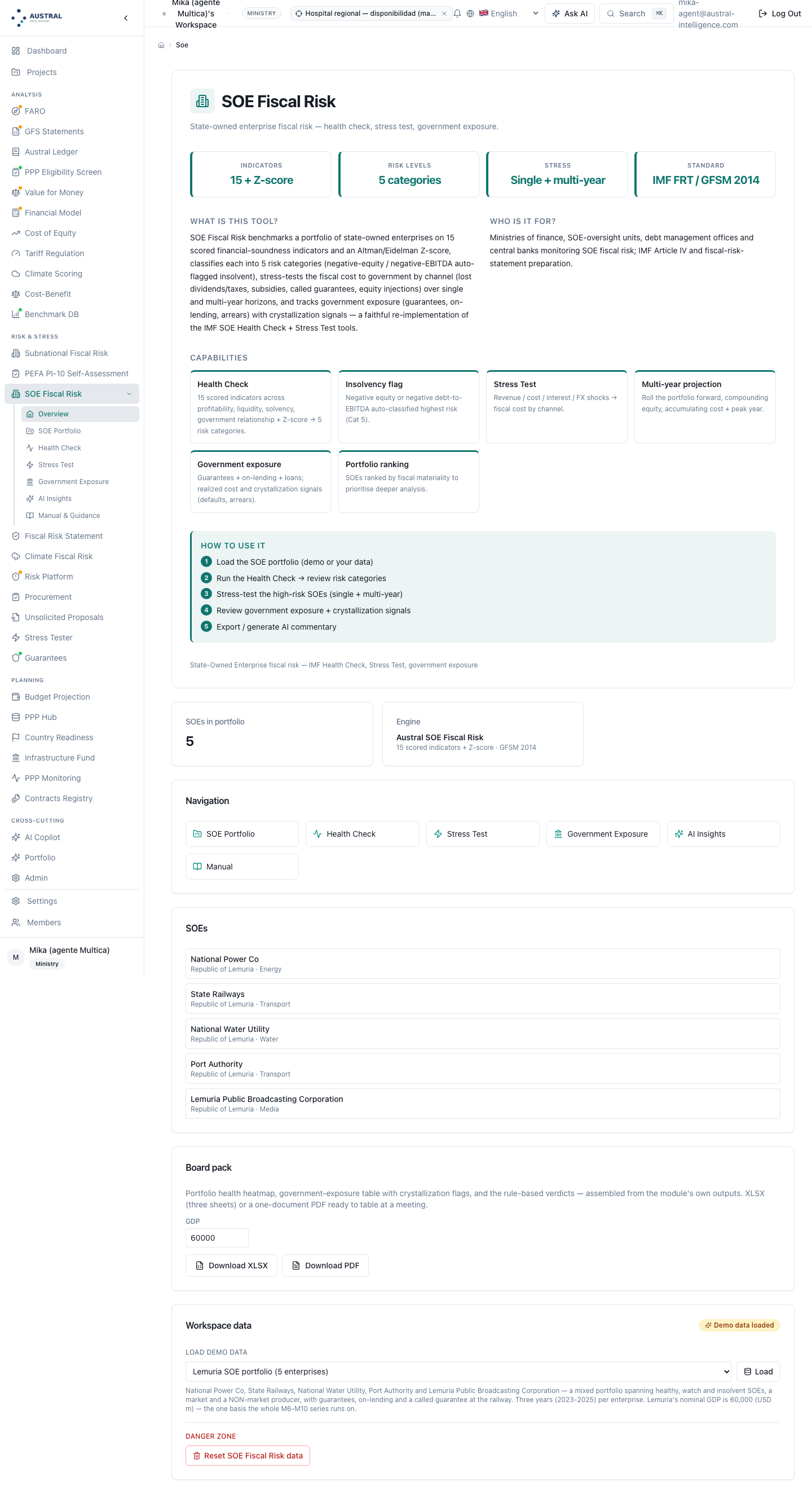
Mandatory honesty note. The §5 module today does issue the market/non‑market classification as a binary decision per enterprise, with its ratio, its window and its note, and for the non‑market enterprise it publishes the total stock of liabilities as direct debt alongside the guaranteed stock, both labelled; and it evaluates the Step 0 perimeter with the ownership share and three explicit control flags. The two steps this section described as not run by the tool are in fact run, and §5 says where the execution still falls short — neither the board pack nor the consolidated register yet carries the classification or the perimeter, consolidation does not read the perimeter test's result, and there is no surface for calibrating the thresholds and weights or for building §3.4's two‑axis reading. This is stated here, in the section where the manual credits its sources, because the alternative — describing the full method and letting the reader assume which part the tool runs — would be exactly the useful silence the house criticizes in its own papers.

2.8 Correspondence table: §3 step → source → §5 screen

Figures marked with ◆ are engine defaults, configurable on each run; they do not come from the cited source but from Austral's calibration, and §3 publishes them so the reviewer can dispute them. The reverse table — from screen to step, including the steps that today have no screen — is in 5.1.

3. The method, step by step

Ten steps, from the perimeter to monitoring. Each one declares what goes in, what comes out and what the rule is — the rule is what makes the step reproducible by another analyst with the same data. The method is written to run with any tool: a spreadsheet and a folder of evidence are enough, and that is the condition that later lets §6 show where that spreadsheet breaks. Where the §5 module's practice departs from the source, or where it does not yet run the step through to the end, it is said at the step and repeated in §5.

A reading convention that governs all ten steps: a data point that does not exist is not a zero. Unreported revenue, a blank finance cost, an unreported guaranteed stock are left empty, and every indicator that needs them returns N/A and is counted as a data gap. Writing a zero is asserting that the figure is zero, and none of the rules that follow work if that distinction is lost.

Step 0 — Perimeter: which enterprises come in

In: the universe of entities in which the State has ownership, a stake or influence — the list kept by the entity exercising State ownership, the budget's enterprise annex, the register of State corporations, and entities none of those three lists contains but that the State controls some other way.

Out: the list of SOEs within scope, each with its inclusion basis written down — why it is in — and the consolidation basis that applies to it; and, alongside it, the list of those left out, each with its reason. The second list is as much a part of the deliverable as the first (§1.5, figure 6).

The rule is four cuts, in this order. Order matters: each cut assumes the previous one has already been applied, and skipping one produces errors that are not caught later.

0.1 Is it a resident institutional unit?

Before asking who controls it, one has to ask whether it is a unit at all. An entity that cannot make economic decisions on its own account, does not keep a full set of accounts, and cannot incur liabilities in its own name is not a separate institutional unit and is not diagnosed separately: it is classified together with the unit that controls it. Two frequent cases, both covered in the statistical rulebook (§2.4):

• An artificial subsidiary — a paper company that only holds its parent's assets or debt, with no capacity to act independently — is consolidated with its parent and does not enter the portfolio as its own row. If it does, its debt is counted twice.
• A central borrowing authority that raises debt in the market and only lends to its parent or to other general‑government units is classified within general government, even though it looks like a public financial corporation. It is not an SOE for the purposes of this method.

And residence: a subsidiary incorporated abroad is a non‑resident unit and does not enter the national portfolio, even if the parent is State‑owned; what enters is the parent's stake in it.

0.2 Is it controlled by the State?

Control is not a majority shareholding. The definition the method uses has three elements that must all hold (§2.4): the State (a) has power over the entity — existing rights that give it the current ability to direct its relevant activities; (b) is exposed to variable benefits from its involvement with it; and (c) has the ability to use that power to affect the nature or amount of those benefits.

In the public sector, power rarely comes from voting. The usual routes, which are the ones to look for in the charter and in agreements:

Three limits that avoid a false positive, and that are worth writing into the report because they are what the comptroller's office asks: regulation is not control — a sovereign power applied to a whole industry does not give control over one enterprise in it; economic dependence is not control — a single customer, however large, is not enough on its own; and protective rights (vetoing a change of corporate purpose, approving a debt issue that would jeopardize the investment) are not power. Conversely: a law declaring that the enterprise operates with autonomy does not by itself rule out control.

The decision is made on the totality of the evidence, is necessarily a judgement, and the method therefore requires two things: that the judgement be written down with the evidence behind it, and that similar cases be decided similarly — a criterion applied to one enterprise and not another turns the perimeter into a preference.

Output of this cut, per enterprise: inside the perimeter / outside / not evaluable, with the basis (ownership share, or the explicit evidence that substitutes for it) and the consolidation basis: full consolidation for the controlled entity; the equity method for significant influence without control; financial investment for the rest.

Austral's convention on control that cannot be evaluated. The third outcome — not evaluable — exists and is used: there are entities for which the register has neither a declared ownership share nor explicit evidence of any of the routes in the table above. Austral's convention, declared as such, is that the entity is fully consolidated and is named, by name, in the warnings of the run and the report.

It is the conservative fiscal reading: if it is not known whether the State controls the entity, the assumption is that it does, and the entity enters in full, because the error of leaving out a balance sheet the State does own is more expensive than including one it does not. And it deliberately runs against the grain of the accounting consolidation standard, which requires positive evidence of control before consolidating and, in doubt, would leave the entity out.

Both things are stated together whenever the convention applies: it is an Austral choice, not a rule of the standard, and the affected enterprise is named so the reader can reverse it. A perimeter that expands silently is as bad as one that shrinks silently; what the method forbids is the reader not knowing which of the two happened, and to which enterprise. §5 shows how this looks in the product.

0.3 Is it financial or non‑financial?

State banks, deposit‑taking institutions and development banks fall outside the method and are declared out. This is not an omission: their statements take a different shape and their diagnosis needs other indicators — capital adequacy, portfolio quality, sensitivity to market risk — and applying Step 3's fifteen indicators to them produces a rating that looks like a result and is not one. A State bank with a fragile solvency ratio could come out Cat 1 under this method.

In scope: non‑financial public corporations, including those in utilities, transport, energy, water, telecommunications and media. Out of scope, and declared as such: financial enterprises, public pension funds, and special‑purpose vehicles whose only function is financial.

0.4 Which level of government?

Central‑government enterprises, and regional‑ and municipal‑government ones, are not mixed without saying so. They can be analyzed together — the method is the same — but the register has to be able to separate them, because the figure that goes into the central government's fiscal risk statement is not the same as the public sector's, and because the recipient of the risk differs in each case.

What is not an entry criterion

Whether or not the enterprise has State‑guaranteed debt. It is the most common shortcut — the register gets built from the list of outstanding guarantees — and it is exactly the error §1.6 describes: it produces a portfolio biased toward enterprises that asked for a guarantee, which are not the riskiest ones but the ones that could not borrow without it, or the ones that arranged it first. The insolvent enterprise with no guarantees does not show up in that register, and it is the one that is going to cost money.

Method note. The control test is a decision with accounting and statistical consequences. The fiscal analyst applies and documents it; who fixes it formally is government accounting and the statistics office. The register records who decided it, and when (Step 9).

Step 1 — Inventory and financial statements

In: for each enterprise from Step 0, descriptive data and an abbreviated set of financial statements, one row per year.

Out: the enterprise record with its three blocks complete and its data gaps declared.

1.1 The three blocks

(a) Descriptive data. Name, sector, country, State ownership share and Step 0.2's control flags (board control, golden share, contractual control), because the ownership share alone does not decide the perimeter, and the register has to be able to tell a 30% associate with a golden share apart from a 30% associate without one.

(b) Income statement and balance sheet, abbreviated, under International Financial Reporting Standards or a similar format:

Two warnings about that table, because they are the two that produce the most errors.

• Depreciation and amortization appears twice, and it is not an error. It sits inside "other operating expenses" — which is how almost every statement reports it — and it is also declared separately, because the method needs it to add back EBITDA (EBITDA = EBIT + depreciation) and to avoid inflating it when Step 6 applies a cost shock. Declaring it in only one of the two boxes breaks either the EBITDA figure or the cost shock, and neither error is visible on screen.
• Explicit subtotals override the sum of components. If the analyst enters total assets, that is what is used; if not, it is summed. This is deliberate: a real statement rarely reconciles exactly with the sum of the abbreviated lines, and forcing it to would invite forcing one line to fit.

(c) The transactions‑with‑government block. This is Step 5's exposure record, and the part no financial statement brings ready‑made; it has to be built with the debt office and the budget office:

The distinction between a capital transfer and a capital contribution is Step 5's, and the source sets it (§2.1): a capital transfer is one for which no market return is expected; a capital contribution is one for which shares are issued, a market return is expected, and the government recognizes it as the acquisition of a financial asset. Entering them in the same box erases the only information that later allows a decision on whether the outlay was an expense or the acquisition of an asset.

1.2 Step 1's rules

(a) Sales revenue never includes government transfers. It is the most consequential rule in the whole method, because it is the one that decides Step 2. An operating subsidy, a contribution to cover a deficit, a social‑tariff compensation entered into the revenue line make an enterprise that fails the 50% test pass it, and the reclassification does not happen. The fix is not in the formula: it is in the input form, by separating the line. And there is a middle case Step 2 resolves, not Step 1: a government payment tied to the volume or value of output — a per‑ticket subsidy — is a sale; a lump‑sum payment to cover an operating deficit is not.

(b) The statements have to reconcile. Two identities, and the method checks them before calculating anything:

net income = EBIT − finance costs + finance income − income tax EBIT = commercial revenue + other operating revenue − cost of sales − other operating expenses total assets = total liabilities + equity

A statement that does not reconcile gets fixed or flagged. This is not a cosmetic requirement: Step 6 takes the dividend payout ratio from reported income and applies it to its own recalculated income, so a net income entered as a headline — rather than derived from the lines above — makes the model destroy more dividends and taxes than the State actually receives. §6.3 tells that story.

(c) All available years are loaded, not just the latest. Step 2 is a window test and Step 3 has a trend reading; neither works with a snapshot. The operational minimum is three years, which is the window the statistical source requires for classification (§2.3); the Health Check source allows up to fifteen. With a single year the method still runs, but Step 2's classification is flagged provisional and there is no trend reading. Declaring the window used is part of the result.

(d) The data gap is declared. At the close of Step 1, the record lists which indicators will be left N/A for lack of input. That list is what later makes it possible to read Step 3's weighting coverage and decide whether that enterprise's rating is publishable.

Step 2 — Classify: market or non‑market

In: from the declared window, the series of own revenue and production costs for each enterprise, plus the qualitative background from Step 0.

Out: a binary decision per enterprise — market / non‑market / not evaluable — with its ratio, the years actually used, and a note explaining the result.

This is the manual's hinge. It is written before the Health Check, not after, precisely so the reader does not think the risk rating is what decides the perimeter. They are two different questions: Step 3 says how likely is the enterprise to generate fiscal cost; Step 2 says whose debt is it. An enterprise can be Cat 2 — healthy — and non‑market, with its entire debt being debt of the government.

2.1 Qualitative conditions first

The qualitative conditions take priority over the ratio, and failing a single one is enough to classify the unit inside general government without applying the quantitative test (§2.3). There are four:

1. Is it an institutional unit? (already resolved in Step 0.1).
2. Is it not a captive supplier of ancillary services to government? An entity that exists to provide an internal service to the State — transport, maintenance, IT — is not a market producer no matter how much it bills.
3. Is it not the government's sole supplier, or, if it is, does it compete with private producers? If the only outlet for its output is the State and the choice of supplier is not made on price, it is not a market producer.
4. Does it have an incentive to adjust its supply to run a profitable, viable activity and to meet its financial obligations? This is the soft‑budget‑constraint question, and the indicator that tilts it is the one the source names expressly: an enterprise that receives substantial financial support from government, or that enjoys substantial State guarantees, responds to economic conditions differently from one that does not, and is more likely to be classified as non‑market. Read the direction carefully: under the statistical rulebook, a State guarantee is an argument for taking the enterprise out of the public‑corporations sector, not a substitute for the test.

Each is answered yes / no with its evidence. A "no" closes the step with a non‑market classification and a note stating which one failed.

2.2 The ratio, with the orientation the method uses

Once the qualitative conditions are cleared, the ratio between production costs and sales is calculated:

ratio = (cost of sales + other operating expenses + finance costs − finance income) ÷ (commercial revenue + other operating revenue)

Note the orientation: costs over sales, so that lower is better and the line "sales cover half of costs" falls exactly at a ratio of 2.0. A ratio of 2.0 means costs equal to twice own revenue; above 2.0, the enterprise fails the test.

Three points that decide the result more often than the arithmetic:

• The net interest charge enters production costs. This is the European convention, which is the one this method follows on accounting figures; the Fund's statistical manual puts a return to capital there instead, and neither one puts both (§2.3).
• The zero floor on the net interest charge: the rule, and what the engine does today. The MGDD ¶53 requires that when the net charge comes out negative — an enterprise with more finance income than finance costs — it be replaced by zero rather than subtracted. The Health Check Tool's formula carries no such floor (figure A2.4, p. 21), and the §5 engine reproduces the tool's formula: today the floor is not applied. The difference only shows up in enterprises with a net creditor financial position, and always in the same direction — without the floor, the ratio improves and the enterprise moves closer to "market." Until the register fixes the convention, Step 9's presentation rule applies: the ratio is published stating which formula calculated it, and enterprises whose finance income exceeds their finance costs are flagged, because they are exactly the ones where the two sources would give different numbers.
• Government transfers are excluded from sales, except those directly tied to the volume or value of output that would be granted to any producer in the same activity. The per‑ticket subsidy counts; the lump‑sum contribution to cover an operating deficit does not.
• Holding gains, dividends received, investment grants and other capital transfers do not enter sales.

2.3 The window: how it is summed

The test is sustained, not one year's. And how it is summed matters:

The window's costs are summed, and the window's sales are summed, and one sum is divided by the other. Ratios are not averaged year by year.

The difference is not cosmetic. Averaging ratios lets one year of abnormally low revenue — a strike, a shutdown — dominate the average and reclassify an enterprise that does not deserve it. It is worth being precise about where the rule comes from: none of the sources write how the window is aggregated. GFSM 2014 and the MGDD ask for a range of years to be looked at; note 6 of the Health Check Guide (pp. 24‑25) asks to "look at several years of data (ideally a minimum of 3 years' financial results)." Summing the flows rather than averaging the ratios is, therefore, an Austral convention, declared as such: it is the reading consistent with the idea of a sustained period, and it is what the engine applies.

The timing rules, which are what prevent flip‑flopping:

• The unit stays outside government only when the test holds for at least three years.
• Conversely, if the unit did not pass the test in one year and is expected not to pass it in the next two, it is classified immediately inside government.
• A minor fluctuation or an exceptional result does not reclassify: only a change in pricing that holds, or is expected to hold, for several years justifies revisiting the classification.
• A new enterprise, with no history, is classified on a realistic business plan, and the classification is flagged as such until there are three years.

And the honesty rule: with a single year of statements, the classification is provisional and is published flagged as provisional. It is not "market with one year"; it is "provisional, pending a window."

2.4 The complementary test when the ratio sits close to the line

A ratio between, say, 1.7 and 2.3 does not decide anything on its own: it is within the measurement error of abbreviated statements, depreciation conventions, and the classification of a single line item. For those cases the method adds a complementary test, which is the operationalization The Anchor and the Perimeter applies to Chile's twenty‑eight State enterprises (§2.7):

An enterprise is classified non‑market if, over the window, cumulative EBITDA is negative; or if there are persistent losses and dependence on recurring Treasury contributions — transfers or capital contributions in most of the window's years, without which the enterprise would not have covered its debt service.

Worth stating what this test is and is not. It does not reproduce the sales‑over‑production‑costs arithmetic: it is a cash‑generation and dependence criterion, built on public information, that arrives at the same place by another route. The manual uses it as a declared tie‑breaker, not a substitute, and the register states which of the two operationalizations decided each case.

2.5 The consequence, which is the step's point

The non‑market enterprise's two readings are published together and labelled, and are not added: the guaranteed stock is a subset of the total stock, not an addend. It is the easiest double‑counting error to make in this step.

Why three years and not five. The method's default window is three years, and it allows up to five when data exist, on a "most recent" basis. Five as a default would produce more stable, slower‑reacting classifications; three is the minimum the source requires and the one most registers can sustain, which is the reason for the choice.

Step 3 — Health Check: the fifteen indicators and the five categories

In: Step 1's statements and Step 3.1's threshold and weight set.

Out: per enterprise — the value and Cat 1‑to‑Cat 5 category of each indicator; the two margins reported unscored; the Z‑score with its band; the insolvency flag; and the overall weighted rating with the weighting coverage it was built on.

3.1 The fifteen indicators

Four groups. The threshold column is the source's illustrative set (figure A2.5, p. 22 — §2.1), which is a starting point and not a standard: see 3.3.

Fifteen with a threshold, thirteen in the rating. All fifteen have a band in figure A2.5, and all fifteen are published with their category. But the source's selection screen — figure A2.6, p. 28 — offers only the profitability, liquidity and solvency ones for the weighted rating: thirteen. The two relationship‑with‑government ones have a threshold and no box. It is not that the source gives them zero weight: it simply does not put them in the mechanism. That is where 3.4's two‑axis reading comes from, and why Austral's fiscal‑use weight set is not a recalibration within the source but a declared extension of it.

Profitability (3 indicators)

‡ These are the thresholds figure A2.5 prints and the ones the engine applies. The same Guide's reasoning (p. 22) explains them with different numbers — the local stock market's average return for Cat 1, "assumed to be 15 percent for illustrative purposes," and the ten‑year risk‑free rate for Cat 2, "assumed here to be 8 percent." The text and the table do not agree; the manual publishes the table and uses the reasoning for what it is good for, which is saying where the cut should come from when calibrating by country (3.3).

Cost recovery uses revenue without transfers: it is the enterprise's own operational break‑even point. Below 1, the enterprise does not cover its operating costs with what it sells.

◆ The Cat 3 cut for return on assets, 0.05, is an Austral calibration and not the source's: the published table prints the same number for Cat 3 and Cat 4 — 0.1 · 0.0 · 0 · (0.1), figure A2.5, p. 22 — which leaves the Cat 3 band empty and produces a two‑category jump around zero. Austral opens it by mirroring, at the halfway point of the scale, the return‑on‑equity ladder, which is the derivation the Guide itself declares for this indicator — "the risk thresholds have been determined based on the risk thresholds for ROE and balance sheet leverage" (p. 23): half of 0.10 is 0.05. Even with that support, the cut is attributed to Austral, because the published table does not print it. It is declared here, in §2.1 and in §5 (§2.8).

Liquidity (4 indicators)

Days payable are calibrated higher than days receivable on purpose: good working‑capital management collects before it pays. A very high days‑payable figure is not efficiency, it is trade arrears.

Solvency (6 indicators)

A note on naming. The first three are calculated on total liabilities and the last on interest‑bearing debt. The source labels all of them debt to … / debt coverage, so the ambiguity between "debt" and "liabilities" is the source's, not the implementation's, which reproduces it exactly. This manual calls them "liabilities to …" wherever the numerator or denominator is total liabilities, because a fiscal‑risk reader who reads "debt to assets" and calculates financial debt will get a different number. The Cat 5 cut for liabilities to assets sits at 1.00 for a reason worth spelling out: liabilities above assets is negative equity.

Relationship with government (2 indicators)

The 50% test's Cat 5 cut is exactly Step 2's line. Here it is scored; there it is decided. It is the same number with two different uses, and the manual does not confuse them: an indicator in Cat 5 lowers a rating; a non‑market classification moves a stock of debt.

The two reported margins, and the Z‑score

Net margin (net income ÷ own revenue) and operating margin (EBIT ÷ own revenue) are calculated and reported unscored, because the source sets no threshold for them: they are trend and sector‑comparison indicators. Reporting them with an invented category would be attributing a threshold to the source it does not have.

The Z‑score is the emerging‑markets variant of distance to default:

Z = 6.56 · (working capital ÷ total assets) + 3.26 · (retained earnings ÷ total assets) + 6.72 · (EBIT ÷ total assets) + 1.05 · (equity ÷ total liabilities)

Its bands are fixed, and the source declares they cannot be adjusted: Z > 2.6 → Cat 2; 1.1 < Z ≤ 2.6 → Cat 3; Z ≤ 1.1 → Cat 4. Note there is no Cat 1 or Cat 5: the Z‑score's scale does not cover the extremes of the risk scale, and reading it as if it did is a mistake. The Z‑score needs retained earnings as its own line; without it, it returns N/A, and it is the method's most frequent data gap.

3.2 Step 3's four rules

(a) An indicator with no input returns N/A and is not scored as zero. A zero is a data point; an absence is not. Scoring the absence as zero artificially lowers a rating; silently ignoring it raises one. The correct output is N/A, and the consequence is in rule (c).

(b) The insolvency guard, with two levels that must not be confused.

The source states the guard in one sentence and about one thing only: "for any entity that has negative equity or a negative debt to EBITDA indicator, the indicator is automatically classified in the highest risk category (Category 5)" (Health Check Guide, §IV.A, p. 8). That is, the source's guard operates on the indicator. The method adds two things to it, and both are Austral conventions, flagged below.

• Negative equity forces Cat 5 on the two indicators that divide by equity — return on equity and liabilities to equity — which is the source's guard, and it additionally forces Cat 5 on the entity's overall rating — which is not in the source: it is an Austral convention — above the weighted average. A technically insolvent entity cannot escape the maximum risk category because the average of its other indicators pulls it down. The numeric overall rating is not altered — it remains real information about the other indicators; what is forced is the category, and the register notes why it was forced.
• Negative EBITDA forces Cat 5 only on the liabilities‑to‑EBITDA indicator, the one that divides by EBITDA. It does not by itself force the entity's category: it pulls the average up like any other Cat 5. The source phrases the trigger as "negative liabilities‑to‑EBITDA indicator," which with positive liabilities amounts to the same thing, and the method uses that phrasing.

And a second Austral convention, on presentation, which matters more than it looks and which the source also does not write: when the negative‑equity guard fires, the ratio's value is not printed. Negative income divided by negative equity gives a positive return; positive liabilities divided by negative equity give a negative number that reads as "moderately leveraged." Both are arithmetically correct and neither is interpretable. The category — Cat 5, by the guard — already carries the whole signal; the value can only mislead.

(c) The overall rating is renormalized over the evaluable indicators, and is published alongside the weighting coverage. The source says two things, and only two: that the weights of the selected indicators sum to 100%, and that the overall rating is the weighted average of their categories (Health Check Guide, §IV.B, p. 8; annex II.D, p. 28). It does not say what to do when a selected indicator cannot be evaluated. What follows — renormalization, publishing the coverage, and the rounding rule — is an Austral convention.

overall rating = Σ (indicator weight × its category) ÷ Σ (weights of the evaluable indicators)

N/A indicators are excluded from the numerator and the denominator. That is correct, and it is also the gap: an enterprise with almost no data produces a rating built on a tiny fraction of the expected weight, and that rating looks exactly like a complete enterprise's. The method's rule:

The weighting coverage — the fraction of the expected weight actually used — is published alongside the rating, always. A rating built on 15% of the weight is not a rating; it is a missing data point shaped like a number.

The overall category is obtained by rounding the rating up on a tie (2.5 → Cat 3, not Cat 2) and capping it to the 1‑5 scale: in a supervisory rating, a tie resolves toward the higher risk. This too is an Austral convention — the source sets no rounding rule — and it is declared because it changes the published category of roughly one enterprise in several dozen.

(d) The Z‑score is read as a contrast, not a vote. It does not enter the weighted rating. It is a corporate‑credit indicator taken from the financial literature, not calibrated for SOEs — an SOE can have a terrible Z and service its debt without trouble because its owner will not let it fail, which is precisely the fiscal risk this manual measures. Its usefulness is in the discrepancy: when the Z and the weighted rating say different things, there is something to look at. When they agree, it added nothing new, and it does no harm either.

3.3 Calibrating the thresholds

The illustrative set is a starting point, explicitly declared as such by the source: "an illustrative set of thresholds […] which could be used for in the SOE HCT, in the absence of more robust datasets" (Health Check Guide, annex II.C, p. 22). The same current ratio means different things at a port and at a railway, and in one country and another. Using it without calibration is not a methodological error — the source allows it — but it is a decision that has to be declared.

Four calibration routes, and three statistical approaches depending on sample size (Health Check Guide, annex II.C, pp. 22 and 26‑28 — §2.1):

The rule, whatever the route: the threshold set used is published with the result, or the result is not auditable. The same holds for weights. A portfolio of forty enterprises scored against thresholds no one can say where they came from, in an unversioned file, is not a register: it is an opinion with tables.

3.4 What the overall rating does not say

This has to be spelled out because it is counterintuitive, and with a precision stronger than what the manual used to say. In the default weight set, the two relationship‑with‑government indicators carry zero weight — and in the source they cannot carry anything else. The default set splits 100% across seven indicators — return on equity 0.20; cost recovery 0.10; current ratio 0.15; days receivable 0.10; days payable 0.10; liabilities to assets 0.15; liabilities to EBITDA 0.20 — and leaves out the remaining eight, including transfers to revenue and the 50% test. Those seven weights are, one by one, the ones in the Health Check Guide's figure A2.6 (p. 28), checked against it; and that same figure shows that the source's selection screen only offers the thirteen profitability, liquidity and solvency indicators. The two relationship‑with‑government ones have a threshold in figure A2.5 and have no box in A2.6.

This is not a flaw: the source's selection is designed to measure financial soundness. But a fiscal‑risk reader is asking something else, and the two indicators that matter most to them — how much the enterprise lives off transfers, and whether it covers half its costs — do not touch the rating. The overall rating of an enterprise that lives off transfers can come out the same as one that receives none.

Austral's position is a two‑axis reading, not a higher weight. It is the step's rule, not a suggestion:

The overall rating measures financial soundness and is published with the source's weight set, unmodified. Alongside it, and not inside it, the fiscal‑dependence axis is published, with three components and no average of them: the transfers‑to‑total‑revenue category, the 50% test's category, and the Step 2 classification. An enterprise is dependent if Step 2 sectorizes it within general government, or if either relationship‑with‑government indicator falls into Cat 4 or Cat 5; autonomous otherwise. And it is fragile if its overall rating is Cat 4 or Cat 5, sound if Cat 1 to Cat 3.

Every enterprise in the register is therefore published on two coordinates, in one of four quadrants: sound and autonomous, sound and dependent, fragile and autonomous, fragile and dependent. The fourth is the one the State pays for; the second is the one that is going to surprise it. The two coordinates are never averaged together at any point in the method, because they measure different things: one measures whether the enterprise can carry its own balance sheet, the other measures how much of its operation is, in effect, public spending.

For anyone who needs a single number — a ranking, a traffic light, a dashboard row — Austral also publishes a fiscal‑use weight set, explicitly marked as an Austral calibration and not the source's. And it is worth being precise about in what sense it is not the source's: it is not that Austral picks different weights within the Guide's mechanism — it extends the mechanism, because it gives weight to two indicators the source's selection screen does not offer. A user of the Fund's spreadsheet cannot build this set. It shifts a third of the weight to the two relationship‑with‑government indicators and keeps the relative proportions of the rest:

And the set is published with its uncomfortable result in plain view, not with a footnote softening it. Giving weight to the two relationship‑with‑government indicators takes it away from the solvency ones, and that improves the rating of an enterprise that is fragile but autonomous. Measured on §4's portfolio with today's engine: the fiscal set leaves the broadcaster — non‑market, financed by transfers — as the portfolio's worst‑rated enterprise (4.90 versus 4.85), which is what was intended; but it improves the water utility from Cat 4 to Cat 3 (3.55 → 2.92), and the water utility is exactly the enterprise Step 7's projection finds at zero equity under the sustained shock. Its problems are solvency ones and its relationship with government is good, so a weight set that rewards autonomy rewards it.

That result is not a flaw in the set to be fixed by recalibrating: it is the demonstration that a single number does not answer two questions. And it is exactly why Austral's position is the two‑axis reading and not the weight set. The set is offered to whoever needs the number; the manual delivers it with this case alongside it, because publishing it without that would be selling, as a fiscal calibration, something that, in the fragile‑and‑autonomous quadrant, points the other way. §4.4 shows the two axes and the set's effect on the five enterprises.

Step 4 — Prioritize: fiscal materiality

In: Step 3's category, Step 1's stock of liabilities, and Step 2's classification.

Out: the ranked portfolio, and the year's division of work.

The ranking rule is category first, liabilities stock second:

1. Non‑market enterprises from Step 2 go to the top of the list, regardless of their category, because their debt is already government debt and the work they require is not surveillance but accounting and statistical recognition.
2. Then, by descending risk category (Cat 5 first).
3. Within each category, by descending liabilities stock.

Why liabilities, and not revenue, or assets, or headcount. Because liabilities are what the State could end up assuming. An enterprise with huge revenue and a light balance sheet is not a bigger fiscal risk than one with modest revenue and four thousand in debt; and headcount measures a political problem, not a fiscal one. Assets do not work either: a specific fixed asset — railway tracks, a water network — is not realizable and does not cover the liability.

The step's useful product is the quadrant: liabilities on one axis, category on the other. What matters is the large‑and‑at‑risk quadrant, and what has to be resisted is the temptation to work the list from top to bottom. A Cat 5 with two hundred in liabilities is a problem for its ministry to manage; a Cat 4 with four thousand is a budget problem.

And the step has a process consequence the source states expressly: prioritization is not the end of the work, it is how the work is divided. The portfolio diagnosis is the first of two stages; the second is in‑depth analysis of the enterprises the first one flagged, with additional information the abbreviated statement set does not carry — debt contracts with their acceleration clauses, maturity schedules, committed investment plans, regulated tariffs and their formula, collective agreements. The annual register says which enterprises get that work this year.

Step 5 — State exposure and materialization signals

In: Step 1's transactions‑with‑government block, and Step 2's classification.

Out: three figures per enterprise and for the portfolio, a binary flag, and the convention note.

5.1 The three figures, which measure different things

Contingent exposure. The stock of debt with an explicit guarantee, at face value. It is what the State would pay if the guarantee were called in full. It is not an expected loss, and the manual says so every time it publishes the figure — including the statistical source itself, which warns that the memorandum item for guaranteed debt offers no information on the likelihood of the contingency occurring and may overstate the risk.

Direct claims. On‑lent loans and government loans receivable. They are not a contingency: they are a State asset that may not be recovered. They are reported separately from the guarantee because their nature and their accounting treatment differ.

The year's realized fiscal cost, net, with both sides shown:

net realized cost = (current transfers + capital transfers + capital contributions + guarantees actually paid) − (dividends received by the State + taxes paid by the enterprise)

Dividends are counted at the State's ownership share, not in full. And the net figure is never published alone: an enterprise that transfers more to the State than it receives gives a negative net figure, and that is valuable information that gets lost if only the portfolio total is published.

The step's hard rule: the three figures are not added together. The first is a conditional stock, the second a receivable stock, the third a year's flow. A register that publishes "total exposure" by adding all three is publishing a number with no unit.

5.2 The non‑market enterprise

For an enterprise classified non‑market in Step 2, exposure is not the guaranteed stock but all of the liabilities stock, because the unit is sectorized within general government. The register publishes both readings labelled — "direct debt by classification: X" and "of which, formally guaranteed: Y" — and, when aggregating the portfolio, takes the larger of the two per enterprise, never the sum.

There is a presentation consequence worth anticipating: when the register does that, the portfolio's total exposure stops being the sum of the guarantees column plus the direct‑claims column. It is correct, and it has to be labelled, or the reader will try to make the columns add up and conclude the table is wrong. The footnote is mandatory.

5.3 Materialization signals

Three facts, any one of which turns the enterprise from a row into a case:

1. A guarantee called: the State paid principal or interest on the enterprise's behalf.
2. Arrears on an on‑lent loan: the enterprise is not servicing debt the government lent it with funds the government itself borrowed.
3. Arrears on a direct government loan.

When any of these occurs, the risk is no longer a risk. The enterprise leaves the annual calendar and enters monitoring; the flag is published alongside the figure, and Step 9 turns it into an off‑cycle review obligation. A register that reports an enterprise's exposure in the same year it called a guarantee, without distinguishing it from the rest, is treating a fact as a probability.

5.4 The convention on capital contributions

Under the statistical rulebook, a capital contribution expected to earn a market return, for which shares are issued and that the government recognizes as the acquisition of a financial asset, is a financial transaction — it is below the deficit line — and is not an expense. Only the portion covering losses is an above‑the‑line expense. The method's own source makes this distinction on its input form, separating the capital transfer (no expected return) from the capital contribution (expected return).

Treating every capital contribution as fiscal cost is conservative and overstates spending; treating all of it as asset acquisition is optimistic and understates the deficit. The method's position:

The register publishes the gross cost — all support, including capital contributions — and, alongside it, the above‑the‑line cost, which excludes the fraction of contributions seeking a market return. The fraction is declared: it is the analyst's judgement about the enterprise's business plan, not a financial‑statement figure, and a contribution to an enterprise with negative equity is unlikely to be seeking a return. Publishing only one of the two figures, without saying which convention was used, is what makes two registers of the same country in two different years incomparable.

5.5 The implicit guarantee

It is named, not priced. The expectation of a bailout with no clause exists — it is what makes an SOE's unguaranteed debt trade closer to the sovereign than to a comparable private borrower — and the rulebook itself lists it among government's implicit contingent liabilities, with the literal example of "assuming the unguaranteed debt of public sector units" (§2.3). The method argues it with Step 3's own rating — a Cat 5 enterprise with four thousand in liabilities has an implicit guarantee, written or not — and puts no number on it, because valuing it requires a bailout probability distribution this method does not build. Pricing it is M7's job; stating that it exists, and how much balance sheet stands behind it, is this manual's.

Step 6 — Stress test: from shock to fiscal cost

In: a scenario of shocks on the enterprise, and two treatment assumptions.

Out: the income statement and equity under the shock, and the fiscal cost through the five channels.

6.1 The scenario

What the Fund's Guide does here, and what this method does. The Fund's Stress Test Tool shocks the fundamentals — domestic and world output growth, inflation, the deflator, the exchange rate, short and long rates, commodity prices, customer liquidity and solvency, indexation of regulated prices, the sales‑tax rate — almost always additively on the rate of change, and lets the model propagate the effect through the three financial statements and government accounts (Stress Test Guide, §IV.8, pp. 30‑33). This method applies direct percentage cuts to four aggregates. This is an Austral convention, and a deliberate simplification: a portfolio register does not have, enterprise by enterprise, the elasticities the Fund's tool assumes are calibrated. What is lost is the automatic cross‑variable consistency the Guide asks of the scenario — "it is important to design the SS according to an overarching narrative," with the signs of the correlations consistent with each other (note 23, pp. 33‑34) — here that consistency is supplied by whoever writes the scenario, not by the model, and that is why it has to be written down.

Four shocks, plus two assumptions:

How the magnitudes are calibrated, and why the default sets are not a calibration. The Stress Test Guide gives the rule, and this manual adopts it: the shock's size is set "in view of the standard deviation (i.e. the historical volatility) of each variable, and the probability the user wants to attach to the SS" — one standard deviation for an event of 30 to 40% probability, two or three for an extreme event (note 22, p. 33). And it gives a reference worth keeping in view: for market variables, "deviation of levels by more than 10‑15 percent of their baseline values can usually be considered very large shocks." This method's default sets — mild 10/5/10/10%, severe 25/15/30/30%, combined 35/20/40/40% — sit, in their severe and combined tiers, above that band. It is not an error: these are stress scenarios, on the order of the two or three standard deviations the same note allows for extreme events. But they are an Austral convention, not a calibration, and in a live run they are replaced with the historical volatility of each variable in the country. A report that publishes the default set without saying this is presenting an assumption as a measurement.

A modelling detail that looks minor and is not: the cost shock does not inflate depreciation. Depreciation and amortization is not a cash cost and does not depend on input prices: it depends on historical fixed assets. Inflating it with the shock breaks the identity EBITDA = EBIT + depreciation and oversizes the subsidy channel, because the subsidy is calculated on the operating cash deficit. That is why Step 1 asks for depreciation to be declared separately: it is what allows the shock to be applied only to the cash portion.

And another: the guarantee's trigger is interest coverage below one, measured with the enterprise under shock — stressed EBIT divided by stressed finance costs. If there are no finance costs, there is nothing to stop paying, and the guarantee is not called.

The trigger is also an Austral convention, and the Guide uses a different one. The Fund's tool does not trigger support through interest coverage: it triggers the capital contribution when the enterprise fails a quick‑ratio floor and a liabilities‑to‑equity ceiling, and only after exhausting, in that order, its own cash and whatever new debt its leverage still allows; the contribution is the residual (Stress Test Guide, §VIII, pp. 60‑61). Both constructions are defensible and are not the same. Austral's has an operational advantage — it can be calculated with abbreviated statements, which is what a portfolio register has — and its cut matches the Health Check's Cat 5 cut for interest coverage (figure A2.5, p. 22). It also has a declared bias: the Stress Test Guide places high interest‑coverage risk a little earlier, at 1.2 (§XI, p. 77), so a trigger at 1.0 is the later of the two and understates how often the guarantee would be called. Anyone wanting the Guide's reading runs the scenario with the trigger at 1.2 and publishes both figures.

6.2 The five channels

The five channels are the ones the Health Check Guide lists in its §I (p. 3). The Fund's stress‑test tool orders them differently on its government‑relations sheet — revenue: taxes, dividends and interest on government loans; expense: subsidies and the fraction of capital contributions that goes above the line (§X, pp. 72‑74) — and publishes the net total to the budget with and without transfers. The correspondence is direct except at one point: a called guarantee is not an expense channel on the Guide's sheet, which treats the guarantee as a contingent‑liability stock and not as a flow; this method counts it as a flow when it fires, which is what a budget sees.

The five channels are always declared separately, and the total is never published without its breakdown. Two of them are revenue that stops coming in and three are expenses that go out, and a minister reads them differently: foregone revenue affects the result but requires no cash or budget authorization; an expense does. A "fiscal cost" total with no breakdown forces the reader to guess its composition, and the guess is always wrong.

6.3 The four rules that order the step

(a) Incremental, not level — and the zero invariant. The shock's cost is the difference against the path of the same enterprise with no shock, not against zero or against a hypothetical healthy enterprise. Worth stating that this comparator is a choice, and what the Guide's is: the Fund's tool also evaluates every indicator in a no‑bailout counterfactual — the same enterprise, the same scenario, with the liquidity gap covered entirely by new debt instead of a capital contribution (§VIII.3, pp. 64‑66; §XI, pp. 76‑78) — which answers a different question: how much does it cost the State to bail out, versus not. Both readings are useful, and this method uses the first; the second is the one to run when the discussion is whether the support is granted at all.

A scenario of zero shocks has to give exactly zero fiscal cost. That invariant is the proof the model is correctly built, and it is run before presenting any result.

If a zero‑magnitude scenario does not give zero, the model is measuring the level and calling it a shock, and every figure it produces will be inflated by the enterprise's structural cost.

(b) Gross alongside incremental, always, in the guarantee channel. Here is rule (a)'s uncomfortable consequence, and it has to be said out loud because it is the one that destroys a report's credibility if discovered later: for an enterprise already failing interest coverage in the baseline, the guarantee is called in both worlds, and the incremental channel comes out zero. The portfolio's worst enterprise shows up with "guarantee cost: 0."

The fix is not to abandon the incremental reading — which is the correct one for measuring the shock's effect — but to publish both figures together:

Guarantee called under the scenario (gross): X. Increase attributable to the shock: 0. The difference is live exposure that materializes with or without the shock.

That sentence, literally, is the one to write in the report. "Zero guarantee cost for the insolvent railway" is the sentence a legislator reads out loud.

(c) No double counting between channels. The subsidy first finances the operating cash deficit; the capital contribution covers only the solvency gap remaining after the subsidy. Calculated separately and added, the same loss gets paid twice.

(d) Both revenue channels are capped.

Foregone dividends and taxes cannot exceed what the State actually receives from that enterprise‑year — that is, exactly Step 5's figures.

It is easier to break than it looks: the payout ratio comes from reported statements and is applied to a recalculated income, and the tax comes from an assumed effective rate rather than the reported charge. Both wedges are routine in real statements — extraordinary items, deferred taxes, non‑controlling interests, equity‑method results, an effective rate that is not the assumed one — and neither is bounded by construction. A model that destroys more income than exists is not being conservative; it is being false, and it also contradicts Step 5 of the same register.

(e) The exchange‑rate revaluation is charged once, on the level. The loss from revaluing foreign‑currency debt is a balance‑sheet charge from the exchange‑rate jump: it happens when the exchange‑rate level moves, not every year the level stays high. The higher finance cost, by contrast, is recurring: foreign‑currency debt that is more expensive in local currency costs more interest every year. Confusing the two multiplies the exchange‑rate channel's cost by the number of years in the horizon.

Step 7 — Multi‑year projection

In: Step 6's scenario repeated over the horizon, the baseline path, and the GDP path.

Out: fiscal cost by year and by channel, the cumulative figure, the peak year, each enterprise's equity path, and the cumulative figure as a percentage of GDP.

7.1 How the projection is run

The baseline grows at a declared rate — revenue and costs, which can grow at different rates — and the year's shock is applied on top of that grown baseline. Two shock paths, to choose from:

• Sustained: the full magnitude every year. It is the "the problem does not get fixed" scenario.
• Declining: the magnitude falls linearly from the first year to a declared floor in the last one. It is the recovery scenario. With the floor at zero, the last year is a zero‑magnitude scenario, and its cost has to be zero — which turns the declining path into a free check of Step 6's invariant.

Both are run and both are published, and that is the step's rule. The path is not a technical parameter the analyst picks once: it is the assumption that decides the headline. With the same portfolio, the same initial shock and the same GDP, §4.6's example gives 13.48% of GDP cumulative if the shock is sustained and 7.22% if it decays to zero — and under the second path, the first path's most‑cited finding disappears: the apparently healthy enterprise that reaches zero equity. Publishing only one of the two is not simplifying: it is choosing the conclusion.

A multi‑year headline is published with its decay rule declared and with at least one alternative path alongside it. The rule is written in one phrase — "linear from full magnitude to zero in year 5," "sustained," "with a floor at 40%" — and justified in another. Year 1 coincides across the two paths by construction, so the only thing separating them is the persistence assumption, which makes the comparison legible.

Modelling assumptions that must be declared because they are choices, not data:

• The debt stock, the guaranteed stock and the foreign‑currency share stay at the base year's level. No endogenous new borrowing is modelled. This is a conservative simplification in one sense — an enterprise in crisis borrows more — and an optimistic one in another — it does not amortize; it is declared, not hidden.
• Baseline finance costs stay constant, and the rate shock acts on them.
• The exchange‑rate revaluation is applied only to the increment over the level already revalued in prior years (Step 6 rule (e)).

7.2 The rule that makes the projection useful

Equity after State support is carried into the following year.

This is what turns a snapshot into a film. The State finances the cash deficit and recapitalizes the enterprise to zero equity every year; that equity — zero, or whatever is left — is the opening equity for the following year. Two findings follow that a single‑period test cannot produce:

• A chronic loss compounds. An enterprise recapitalized in year 1 keeps costing money in year 5, because support returns it to zero rather than to an equity level that could absorb the next loss.
• The enterprise whose equity reaches zero in year 4 or 5 appears, which in the year‑1 snapshot looks like a trouble‑free Cat 3. It is, almost always, the projection's most telling finding and the reason to run it.

7.3 The peak year and the cumulative figure

The peak year — the one with the highest annual cost — is the figure the budget cares about, because it is the one that has to be financeable. It is published per enterprise and not only for the portfolio, because the two do not coincide and the difference is a policy one: the portfolio's peak usually falls in year 1, when the exchange‑rate revaluation and the first recapitalization concentrate, while enterprises that are healthy today have theirs in the last year, because their deterioration is cumulative. A ministry that plans around the portfolio's peak is understating exactly the enterprises it can still save. Under the declining path, by contrast, the peak is year 1 for all of them: the damage is up front and the rest is recovery.

The cumulative figure as a percentage of GDP is calculated over the GDP path, year by year, not by dividing the cumulative figure by a single year's GDP. And it is declared for what it is:

It is a sum of several years' flows over a GDP path, not a stock. It is not comparable to a debt‑to‑GDP ratio and should not be shown in the same table without labelling it as such.

The horizon is the analyst's choice and is declared. Five years is the convention for a fiscal risk statement; ten, for a debt‑sustainability analysis. The method fixes neither. The Fund's tool does: it projects over six years (Stress Test Guide, §I.2, p. 6).

Sum of flows or present value: the difference with the Guide, declared. The Fund's tool aggregates the horizon's flows in present value, discounted at a constant rate — the domestic long rate of the year before the projection starts, chosen precisely so the discount does not move with the scenario — and expresses them over that same year's nominal GDP (§X, p. 74, notes 53 and 54). This method publishes an undiscounted sum of flows over the GDP path. It is an Austral convention, and it answers to its recipient: what a fiscal risk statement needs to know is how much budgetary cash would have to be put up, year by year and in total, not what that commitment is worth today. The two figures measure different things, and neither replaces the other. When the recipient is a debt‑sustainability analysis or a comparison with an asset's value, the cumulative figure is accompanied by the present value, with the discount rate declared; the Guide also recommends recalculating it for a range of plausible rates (note 54, p. 74).

Step 8 — Consolidate and report: where each figure gets written

In: the outputs of Steps 2, 5, 6 and 7.

Out: three destinations that must reconcile with each other, and this manual's declared boundary.

8.1 Statistical destination

And the table of debt concepts, worth keeping in view because the perimeter error is the most expensive one in this discipline, and it almost always consists of comparing two different concepts:

Government‑guaranteed debt of a market‑producer SOE is a memorandum item of general government and actual debt of the public sector. Publishing the first as if it were general‑government debt is an error; leaving it out of the public sector is one too.

8.2 Accounting destination

For controlled entities (Step 0.2): line‑by‑line consolidation of assets, liabilities, equity, revenue, expenses and flows; offsetting the controlling entity's investment against its share of the controlled entity's equity; full elimination of intragroup transactions — which is what makes a government's on‑lent loan to its own enterprise disappear, since in the consolidated statement it is neither an asset nor a liability — and the non‑controlling interest presented within net assets/equity, separately, with results attributed to it even when that leaves it in deficit. Uniform accounting policies; consolidation starts when control is obtained and ends when it is lost.

For significant influence without control: the equity method. For the rest: financial investment.

The creation, merger and transfer of SOEs are handled under the public‑sector‑combinations standard, which classifies the transaction as an amalgamation or an acquisition depending on whether either party gains control. This manual names them and does not develop them: they belong to the accounting suite and to M9.

8.3 Budget destination, and the fiscal risk statement

• In the annual budget law: the year's current transfers, capital transfers and capital contributions, with Step 5.4's convention declared.
• In the fiscal risk statement: the SOE portfolio as its own chapter, with exposure, realized cost and cost under stress from Step 6, plus the list of enterprises whose risk has materialized. That chapter is M9.

8.4 The no‑duplication rule with M7 and M9

Three manuals in this wave touch the same guarantee, and the rule that keeps the consolidated register from counting it twice is one of valuation, not inventory:

The consolidated register takes one of the two — M6's stock or M7's expected cost — never both as if they were two separate obligations.

What M6 does not write, and refers out: the valuation of the guarantee (M7), the portfolio risk matrix and the ceiling (M9), and debt‑sustainability analysis (named only). What M6 does write, even though it touches the others: Step 2's classification, because it is what decides whether there is a guarantee to value at all, or whether the entire debt is already the State's.

8.5 This manual's boundary

M6 decides the classification and delivers the figures. Building the consolidated public‑sector balance sheet — which needs non‑financial assets, eliminations beyond the on‑lent loan, and reconciliation with the national accounts — belongs to the accounting suite and to M9. The manual says so and refers out, rather than promising it. The reason is substantive, not one of scope: what makes the fiscal difference is not consolidation but classification, and that is this manual's.

8.6 The disclosure rule

The primary source warns of this, and the method carries it: since SOE risks are, in many cases, implicit, care has to be taken that public disclosure does not increase the likelihood of the risk materializing, or the cost to government if it does. Publishing that an indebted enterprise is Cat 5 affects its cost of funds, and can bring forward exactly the event one was trying to anticipate.

The rule the method derives is not to publish less, but to publish in the right order: the aggregate portfolio and the methodology are always published; the enterprise‑level detail is published once the enterprise has been notified and a plan is in place. A diagnosis that leaks before a response exists is worse than one published with its response alongside it.

Step 9 — Governance, monitoring and updates

In: the previous year's register and the year's events.

Out: the year's register, with the variance explained by cause, the alerts triggered, and the schedule for the next update.

9.1 The versioned register

Every published figure carries, without exception:

• the date of the financial statements it was calculated on;
• the threshold and weight set used, identified by name and version;
• the window used in Step 2's classification;
• the capital‑contribution convention from Step 5.4;
• the scenario and the horizon from Steps 6 and 7;
• who calculated it and who reviewed it.

An unversioned register is not auditable, and its second year is impossible: no one can say whether the portfolio got worse or the thresholds changed.

9.2 The variance explained by cause

At year‑end, each aggregate figure's variance against the previous year is decomposed into four causes, and only four:

The decomposition is the part of the work no team wants to do, and the only one that turns the register into a series. Without it, a 40% increase in the portfolio's exposure cannot be distinguished from a threshold recalibration, and the reader — rightly — stops trusting either figure.

9.3 Alerts and the schedule

• Materialization alert (Step 5.3): a guarantee called, arrears on an on‑lent loan or a direct government loan, opens a case outside the calendar. It does not wait for next year's register.
• Classification alert: an enterprise whose Step 2 ratio crosses the line, or approaches it for a second consecutive year, enters classification review with accounting and the statistics office.
• Insolvency alert: negative equity for the first time.
• Ordinary schedule: the full register once a year, at the close of the statements. Threshold updates, no more than once a year, declared as a method change.

3.10 One‑page summary

Reviewer's checklist

Thirteen questions. Anyone receiving an SOE register for sign‑off can ask for all of them without redoing a single calculation.

1. Does the perimeter have its control test written down, enterprise by enterprise, with the list of exclusions and their reason?
2. Are sales revenue and transfers kept separate on the input form, and not only in the formula?
3. Do the statements reconcile? Net income derived from the lines above; assets equal to liabilities plus equity.
4. Is the 50% test's window declared, and is a classification based on a single year flagged provisional?
5. Does the classification issue a decision, not only a ratio? And does the non‑market enterprise publish its total stock of liabilities as direct debt?
6. Is the threshold and weight set published alongside the result, with its version?
7. Does the rating come with its weighting coverage? Is there any rating built on less than half of the expected weight?
8. Is the fiscal‑dependence axis published alongside the rating, not inside it? If there is a custom weight set, does it come with its effect measured on the portfolio, including cases where it improves a fragile enterprise?
9. Is the face value labelled as a face value, with the warning that it is not an expected loss?
10. Does the stress scenario pass the zero invariant? And does the guarantee channel publish the gross figure alongside the incremental one?
11. Are the income channels capped by the dividends and taxes the State actually receives, and does that figure match the exposure step's?
12. Does the projection declare its decay rule and publish at least one alternative path, with year 1 matching between the two?
13. Does every figure carry the date of the statements, the capital‑contribution convention, the horizon and the author?

A negative answer does not invalidate the register; an evasive one does.

4. Worked example: five SOEs from the Republic of Lemuria

This section runs §3's method — from the perimeter to reporting — over a complete portfolio, with the opening figures in view, the result of each step, and the reading a ministry of finance would take from it. The portfolio is fictitious: the Republic of Lemuria does not exist, and neither do its five enterprises. It is, deliberately, the same portfolio that comes preloaded in the platform's guest workspace, so any reader can open §5's screens and find exactly the numbers on these pages. Annex 4.A says how.

Three reading warnings, before the first figure.

No figure in this section is written by hand. All of them — the heat map's fifteen rows, the stress test's five channels, each enterprise's equity path — come from a run of the engine on this portfolio, and are replaced by running it again. This is a discipline this manual imposes on itself after an expensive lesson from elsewhere in the series: a row copied by hand into an otherwise correct table carried an error through an entire example. When the example is the proof that the method works, the example has to be an output, not a transcription.

This section's three large figures are different things, and are never added together. Exposure (what the State could lose), realized fiscal cost (what it already paid this year), and cost under stress (what it would pay if next year turns out badly) measure three different things, come from three different calculations, and are published separately. In Lemuria they are 3,810, 775 and 2,264. Their sum means nothing, and a report that writes it is badly written.

The example's currency and GDP are declared assumptions. Figures are in millions of Lemuria's currency and GDP is 60,000 — which makes this a medium‑sized economy with a credibly sized SOE portfolio. GDP is not derived from any data: it is a value the analyst types in, which is why every "% of GDP" figure in this manual carries its GDP alongside it. When the reader applies the method to their own country, that number will change and so will every percentage; none of the method's decisions depend on it.

4.1 The portfolio and its assumptions

Lemuria has five State‑owned enterprises, all non‑financial, all with financial statements for 2023, 2024 and 2025. The 2025 statements are the ones shown below; the two earlier years are used by Step 2 for its window and by Step 3 to read the trend.

Table 4.1 — 2025 income statement, in millions

Note that government transfers sit in their own row, in italics, outside sales revenue. This is not a presentation preference: it is the rule that decides Step 2, and the row a badly built spreadsheet adds upward without anyone noticing. §6.2 measures how much that error costs.

Table 4.2 — 2025 balance sheet, in millions

Table 4.3 — Transactions with government, 2025, in millions

Three of the five enterprises have no figure other than zero in the bottom half of this table: their only financial relationship with the State is the guarantee on part of their debt and, in two cases, the dividend they pay it. That asymmetry is the example's story, and it shows up in no risk rating.

The exercise's declared assumptions, in one place, so the reader can change them:

None of these values is a truth; all are choices, and the method requires that they be published alongside the result. Sensitivity to two of them — the weight set and one threshold — is measured in 4.4; sensitivity to the scenario, in 4.6.

4.2 Steps 0 and 1: why these five and not others

The perimeter, run enterprise by enterprise

Step 0 asks who comes in, and does so with three cuts in an order that matters.

First cut: control. Not majority ownership: control, in the sense of the public‑sector consolidation standard (§2.4) — power over the entity, exposure to variable returns from that relationship, and the ability to use that power to affect those returns. Lemuria's five enterprises are 100% State‑owned, so here the cut is trivial, and each record notes the percentage, the absence of golden shares, and the absence of a management contract that would change the result. A trivial perimeter is not a perimeter that was skipped: the record keeps a note of the test, with its basis, because the year a 40% associate shows up with the right to appoint a majority of the board, the question will have a different answer, and the register has to be able to show the difference.

Second cut: financial or non‑financial. Lemuria also has a State‑owned Development Bank, with a loan portfolio of comparable size to the enterprises above. It does not enter this exercise, and the exclusion is declared with its reason: §3's method diagnoses with non‑financial‑enterprise indicators — interest coverage, liabilities to EBITDA, days receivable — and none of them mean anything about a bank's balance sheet, where the questions are capital adequacy, portfolio quality, maturity matching and market‑risk exposure. Diagnosing a bank with these fifteen indicators does not give a bad result: it gives a result that makes no sense, which is worse, because it looks like a result. The bank needs its own exercise, and until it has one, Lemuria's fiscal risk statement has to say there is an exposure there that has not been assessed.

Third cut: level of government. All five are central‑government enterprises. Lemuria also has municipal sanitation and parking enterprises; they are not mixed with these five, and the register says so. The reason is one of legibility, not size: a portfolio that mixes levels of government produces a "% of GDP" figure no one can attribute to a budget.

And what is not an entry criterion: whether or not the enterprise has guaranteed debt. The Port Authority has 60 in explicit guarantees and Broadcasting has 300; if the perimeter were built from the guarantee register, the portfolio would be a different one and — as 4.5 shows — it would lose precisely the enterprise whose problem is not a guarantee.

The record: an enterprise's three blocks

Step 1 asks, per enterprise and per year, for three blocks: income statement, balance sheet and transactions with government. These are tables 4.1 to 4.3. Three loading rules, and what each one produces in Lemuria.

(a) Sales revenue never includes transfers. In table 4.1 the transfers row is separate and in italics. Broadcasting sells 150 and receives 420; if the two figures were added into the revenue line, the enterprise would "bill" 570 and its 50% test result would change. It is the only loading error in this manual that changes an enterprise's classification, which is why it is the first rule.

(b) The statements have to reconcile. Net income is not a headline: it is what the lines above it produce. Across Lemuria's five records, the identity — net income = EBIT − finance costs + finance income − taxes — closes exactly, with no residual, in all five:

A table of zeros looks like a table with no information. It is the opposite: it is the one table in this section a reviewer should demand before looking at any other, because a mismatch here propagates all the way to Step 6's dividend channel through a route nobody watches. §6.3 tells the story of the time this table did not come out at zero.

(c) Every available year is loaded, not just the latest. Lemuria has three years per enterprise. With only one, Step 2 has no window and Step 3 has no trend; section 4.3 shows exactly how much an enterprise's classification changes depending on which of the three years is looked at.

A complete record, read line by line

It is worth walking through one whole record before the method turns it into categories, because half of what there is to know about an SOE is in the record and not in the diagnosis. We take the railway's, which is going to dominate the rest of this section.

The income statement says three things. It sells 900 and receives 350 in transfers: a quarter of what comes in through its top line is not a sale. Its cost of sales (820) plus its other operating expenses (360) add up to 1,180 against 920 of own revenue, so it loses 260 before even touching interest: it is not an enterprise with a financial problem, it is an enterprise with an operating problem that then has a financial one added on top. The 160 in finance costs against an EBIT of −260 are the second layer, and the 120 in depreciation inside other operating expenses are the third: an EBITDA of −140 means the enterprise burns cash operating, before amortizing a single peso of debt.

The balance sheet says one thing, and it is final. Assets 4,400, liabilities 4,800, equity −400. The enterprise owes more than it has. In the diagnosis this is going to trigger the insolvency guard and decide its category above any average; in the projection it is going to decide that the State recapitalizes it every year. And there is a detail of composition the total hides: of the 4,800 in liabilities, 3,300 is long‑term debt and 600 is short‑term, that is, 3,900 in financial debt against 500 in current assets. The current ratio of 0.42 in table 4.5 comes from there.

The transactions‑with‑government block is what sets this enterprise apart from the rest. 1,500 in guaranteed debt — 31% of its liabilities: the remaining 69% carries no guarantee, and yet the State services it all the same in practice, which is the thesis that opens this manual. 300 in on‑lent loans and 200 in direct loans, which are State assets against this enterprise. 350 in current transfers and 80 in capital contributions received this year. And the three figures that are not stocks but facts: 40 in a called and paid guarantee, 25 in on‑lent‑loan arrears, and a capital contribution that already happened. 60% of its debt is in foreign currency, the highest share in the portfolio, which is what makes the exchange‑rate shock hit it harder than anyone else in Step 6.

A reader who stops here already knows everything important about the railway. What the method adds is not discovery: it is comparability — being able to put this record next to the other four, and next to next year's forty — under the same rule — and consequence — turning the record into a figure that enters the budget and the fiscal risk statement.

A note on this section's figures. All are rounded to the unit, except where the decimal matters. Some column sums may differ from the published total by one unit for that reason — the severe scenario's dividend channel, for example, is 202.6 and appears as 203, while its two components appear as 132 and 70. The published total is always what the engine calculates on the unrounded values, not the sum of the printed column.

4.3 Step 2: market or non‑market, the method's hinge

Before rating anyone, the method asks a question that is not one of quality but of belonging: do these enterprises sell, or are they financed? The rule, from government finance statistics (§2.3), is that an enterprise is a market producer when its sales cover at least half its production costs, assessed on a sustained basis. The ratio published is its inverse — costs over sales — so the halfway line sits at 2.00: above 2.00, sales cover less than half, and the enterprise is not a market producer.

Two calculation points the source imposes, and that change the result: the net interest charge enters production costs, and government transfers are not sales.

Table 4.4 — The 50% test, year by year and over the three‑year window

The window's ratio is not the average of the three ratios: it is the sum of the three years' costs divided by the sum of the three years' sales. The difference matters when one year of low sales would otherwise disproportionately inflate an average of ratios. Neither source states which of the two ways of aggregating the window is correct — they ask for several years to be looked at and do not say how to aggregate them — so summing the flows is an Austral convention (§3, Step 2.3), declared as such and consistent with the idea of a sustained period.

Four of the five are market producers. Their liabilities are the enterprises' own; the guaranteed portion is a contingent liability of the State and the unguaranteed portion is not State debt at all. The fifth, Broadcasting, is not: it sells 160 and costs 354 to produce, propped up by 420 in transfers. The consequence is not a bad grade: it is that Broadcasting is sectorized within general government, and its 900 in liabilities — not the 300 guaranteed, the 900 — are debt of the State.

It is worth pausing on the size of that consequence, because it is the largest result a single decision produces anywhere in the method. For Broadcasting, the figure the State publishes goes from 300 to 900: it triples, with not a single line of its financial statements changing and no one renegotiating anything. All that happened is that someone ran the test.

The box the example can teach, and the one it cannot

Box 4.3.a — The trend the window hides, and the snapshot the window itself hides. Broadcasting fails the test with the three‑year window (2.09), and it also fails it with the latest year alone (2.21). But with its 2023 year alone — a ratio of 1.94 — it would have passed as a market producer. Three readings of the same enterprise: the one the rule declares (sustained window, non‑market), the one the latest data point gives (non‑market, with more room), and the one a chosen year gives (market). The method does not allow the third, and not because the analyst is dishonest: because in a register of forty enterprises updated once a year, "whichever year there is" could be any of them.

The opposite reading is also in the table, and it is more uncomfortable. All five ratios get worse every year, without exception: the railway goes from 1.28 to 1.45, energy from 0.72 to 0.82, the port from 0.60 to 0.68. None of the four market enterprises is close to the line today, and yet all four are moving toward it at the same pace, because in all of them costs are growing faster than revenue. That is the kind of finding a single year's snapshot cannot produce, and it is the argument for why Step 1 asks for every year and not just the latest.

Box 4.3.b — What would happen if the railway failed the test. The railway is the portfolio's most damaged enterprise — insolvent, with a guarantee already called — and yet it passes the test with 1.37 over the window. In its latest year it sells 920 and costs 1,338 to produce: its sales cover 69% of its costs, well above the half the rule requires. It is far from the line, and it drifts toward it more slowly than its income statement would suggest, because the transfers that keep it afloat count as neither sales nor costs. It is worth seeing what would happen if it crossed the line, because the counterfactual measures this step's leverage:

2,800 over a GDP of 60,000 is 4.67 points of GDP that would move to the other side of the State's balance sheet through a test that fits in two lines of a spreadsheet. That is the reason Step 2 comes before the Health Check and not after: whoever looks at the risk rating first ends up believing the rating decides the perimeter, and it does not. Here the portfolio's worst enterprise is a market producer and the one that is not has barely 900 in liabilities; the rating and the classification answer different questions, and this example teaches exactly that because they do not coincide.

And a limit of the example, stated out loud. Broadcasting's test is not close to the line (2.09 against 2.00 has room in one direction, but 2.09 is a ratio that two years of better commercial management could cross). The method calls, for cases that sit close, for a complementary test: cumulative EBITDA over the window, and dependence on recurring Treasury contributions. In Lemuria no enterprise falls into that grey zone in an interesting way, so this section cannot illustrate the complementary test with data. It is stated and referred to §3's Step 2, where the rule is written.

4.4 Step 3: the Health Check for all five

Step 3 scores fifteen indicators against the illustrative threshold set (§2.1), assigns each one a category from Cat 1 (lowest risk) to Cat 5, and produces an overall rating as a weighted average. Two guards operate above the average: negative equity or a negative liabilities‑to‑EBITDA indicator force an entity‑level Cat 5, and in that case the ratio's value is not printed.

Table 4.5 — Heat map: fifteen indicators × five enterprises (value and category)

The railway column's two "—" are not missing data: they are the insolvency guard suppressing the value. With equity of −400 and income of −418, return on equity comes out at +104.5% and liabilities to equity at −12.00 — two numbers a reader would read as excellent, and that mean nothing. The engine categorizes them Cat 5 and does not print the value, which is the only correct response: printing it with a warning alongside is trusting that no one reads quickly.

And two margins that are calculated and reported unscored, because the source sets no threshold for them (§2.1):

Reporting them with no category is more honest than inventing a band for them: the reader sees the data point and knows the method did not turn it into a judgement.

How to read the heat map, group by group

Fifteen rows by five columns is seventy‑five cells, and a reader looking at all of them at once reads none of them. The map reads by group, and in Lemuria each group says something different.

Profitability. This is the group that ranks the portfolio at a glance: the port (Cat 1 and Cat 2), energy (Cat 2), water (Cat 3), the railway and the broadcaster (Cat 4 and Cat 5). And it holds the group's most informative indicator for a fiscal reader, cost recovery — sales without transfers over operating costs: 1.52 for the port, 1.27 for energy, 1.11 for water, 0.78 for the railway and 0.47 for the broadcaster. Below 1.00 the enterprise does not reach operational break‑even; two of the five are there. Note that cost recovery and the 50% test are not the same indicator even though they look alike: the first excludes finance costs and carries no sectorization consequence; the second includes them and does.

Liquidity. This is the group where the portfolio is uniformly mediocre, and that is a finding in itself. The three healthy enterprises all have a current ratio in Cat 4 — 1.05, 1.05 and 1.07, all barely above one — including the port, which is Cat 2 on everything else. A ministry reading only the overall rating will say "the port is fine"; the map says the port is fine and that if its billing slips two months it has a cash problem, just like the other two. Days receivable separates the portfolio more sharply than any other indicator: 29.7 for energy against 121.7 for the railway, four times as much. A railway that takes four months to collect what it bills is financing its customers with State‑guaranteed debt.

Solvency. Six indicators, and the group that carries the most weight in the rating. This is where the row that gives away the water utility sits, one its overall Cat 4 rating does not highlight: liabilities to EBITDA at 8.00 and debt coverage at 0.15, both Cat 5. With an EBITDA of 200 and 1,600 in liabilities, the water utility would need eight full years of EBITDA to pay off what it owes, and its EBITDA covers 15% of its financial debt. Its interest coverage, by contrast, is 2.00 (Cat 2) and its cash interest coverage 3.64 (Cat 1): it pays its interest without trouble and cannot amortize principal. It is the exact profile of an enterprise that refinances indefinitely, and the one Step 7's projection finds at zero equity in year five. The two indicators that say so carry, between them, less weight than return on equity in the factory set.

Relationship with government. Two rows, and the cleanest separation in the whole table: four enterprises in Cat 1 and one in Cat 5, on both indicators. Transfers to total revenue run 0.00 · 0.02 · 0.12 · 0.28 and then 0.72; the 50% test runs 0.68 · 0.82 · 0.95 · 1.45 and then 2.21. There is no gradient: there are four enterprises that sell and one that is financed. And these two indicators — the only ones a fiscal‑risk reader would look at first — carry zero weight in the factory overall rating. That is why the method does not force them into the rating but publishes them as their own axis, alongside it: it is table 4.7, and the weight experiment below measures what happens when the opposite is tried.

One last, cross‑cutting reading: the railway's column has twelve Cat 5s out of fifteen, and the broadcaster's has fourteen. These are not two enterprises with a problem; they are two enterprises with every problem at once, which is what distinguishes a struggling enterprise from a decomposing one. The difference between them is not in the heat map: it is that one has 4,800 in liabilities and the other 900, and that one is a market producer and the other is not.

And a limit of the map that has to be declared. All fifteen rows are calculated on the latest year of each record. The years 2023 and 2024 are loaded and Step 2's test uses them, but no scored indicator looks at them: there is no variation column in this map, no reading of "costs are growing faster than revenue" of the kind table 4.4 does show for the classification ratio. An analyst who wants a trend has to run the check on each year and compare the outputs by hand. It is a difference from the reference tool in §2.1, which does have a company sheet with a trend reading, and it is declared as such in §5.7.

The overall rating, and its coverage

Table 4.6 — Rating, insolvency, distance to default and materiality

Weighting coverage is 100% for all five, and that column, which looks decorative, is what makes the five ratings comparable to each other. An enterprise whose record arrived with half its income statement blank would produce a rating built on a fraction of the expected weight: a number that looks the same and does not mean the same thing. §6.4 measures this on this same portfolio — the water utility with a half‑filled record comes out at 3.25, Cat 3, that is, better than its real 3.55, with 60% coverage. The method's rule is that the rating is not published without its coverage.

The Z‑score does not vote; it contrasts. In Lemuria it agrees with the rating on ordering — the railway and the broadcaster at the bottom, the port at the top — and disagrees on level: it places the two worst enterprises in Cat 4 where the rating places them in Cat 5, and moves the energy enterprise from Cat 3 to Cat 2. That is what one would expect from an indicator taken from the corporate‑credit literature and not calibrated for SOEs: it reads the distance to default of a company that funds itself in the market, and none of these five does. Where the Z‑score does add value is when it disagrees sharply and in the opposite direction from the rating: that does not happen in this portfolio, and the manual says so instead of manufacturing a reading.

The insolvency flag overrides the average. The railway has negative equity, and that forces an entity‑level Cat 5 above any weighted average. Here the average already came out at 5.00, and the guard changes nothing; the interesting case is the opposite one, and it has to be said: an enterprise with good liquidity, good days receivable and negative equity can average out to Cat 3 and still be Cat 5. A register that publishes "insolvent: yes" next to a Cat 3 rating is not being nuanced; it is being incoherent.

The two axes: financial soundness and fiscal dependence

Table 4.6's rating answers one question — can this enterprise carry its own balance sheet? — and does not answer the other one a finance ministry needs: how much of this enterprise is, in effect, public spending? It does not answer it by construction, because the two indicators that would answer it carry zero weight in the factory set. §3.4's method therefore publishes two coordinates, not one, never averaged together.

Table 4.7 — The portfolio on both axes

Read this way, Lemuria's portfolio says something the rating column alone does not. The railway and the broadcaster share a Cat 5 rating and sit in different quadrants, and that difference is the entire policy difference: the broadcaster is a public activity funded by the budget that happens to have the shape of an enterprise — its problem is solved by deciding how much the State wants to spend on it — and the railway is an enterprise that sells, collects poorly, and is sinking under 4,800 in liabilities. A ministry does two different things with each.

And the water utility sits in the same quadrant as the railway: fragile and autonomous. It is the quadrant no relationship‑with‑government indicator gives away, and that only solvency catches — the box from which zero equity is reached without ever having asked for a transfer. §4.6 finds it there in year 5.

None of the five falls into the sound and dependent quadrant, the one §3.4 calls "the one that is going to surprise it." Worth saying rather than manufacturing the case: that quadrant is empty in this portfolio, and a real portfolio of forty enterprises almost certainly has it populated.

How much of the rating is data, and how much is choice

This is the question almost no register asks itself, and the example lets it be answered with two experiments.

Experiment 1: the weights. The factory weight set — the source's, checked weight by weight against its figure A2.6 (p. 28) — splits 100% across seven indicators and leaves the two relationship‑with‑government ones at zero: transfers to revenue and the 50% test. And the point §3.1 adds: in the source those two do not even appear on the selection screen, which offers thirteen boxes and not fifteen. For a fiscal‑risk reader, they are exactly the two that matter most. Austral publishes, as its own calibration and declared as such — and one that extends the source's mechanism rather than recalibrating within it — a fiscal‑use weight set that shifts a third of the weight to those two indicators while keeping the relative proportions of the rest:

And the effect on the five enterprises, with not a single input data point changed:

Two of the five change category: the energy company and the water utility. And the result runs in a direction that has to be read slowly and not softened, because it is the opposite of what the name "fiscal‑use weights" promises. The four enterprises that do not depend on transfers improve, because the weight shifted toward two indicators where they do well; the only one that gets worse is the one that depends on transfers, and it barely gets worse (+0.05) because it was already at the top of the scale.

Among those that improve is the water utility, which moves from Cat 4 to Cat 3 — and the water utility is the one §4.6 finds at zero equity in year five. It is the fragile‑and‑autonomous quadrant in table 4.7: its problems are solvency ones and its relationship with government is spotless, so a weight set that rewards autonomy rewards it, and a ministry that prioritized on that column would look at it right after the energy company.

That result is not fixed by recalibrating the weights. It is fixed by not asking one number to answer two questions, which is exactly what table 4.7 says and what §3.4 sets as Austral's position: the overall rating is published with the source's weights and measures soundness; fiscal dependence is published alongside it as its own axis. The fiscal weight set is published all the same — marked as an Austral calibration and not the source's — because some readers need a single‑column ranking, and it is published with this table and this case alongside it. Publishing it without the water‑utility case would be selling, as a fiscal calibration, something that, in one quadrant of the portfolio, points the other way. Publishing it with the case is what lets the reader know which part of the number is the enterprise and which part is the analyst.

Experiment 2: a threshold. The published illustrative set has, for return on assets, a four‑cut ladder in which the Cat 3 and Cat 4 cuts are the same number, leaving the Cat 3 band empty and making the indicator jump two categories around zero. Austral's implementation opens that band with its own cut, declared in §2.1 as an Austral repair and not a source threshold. Its measured effect here:

One enterprise changes category on that indicator and none changes overall rating, because return on assets carries zero weight in the factory set. The experiment is still worth running, and for two reasons: it shows a disputed threshold can have zero consequence for the published result — useful information for deciding what is worth disputing — and it records that the difference between the implementation and its source is one of attribution, not magnitude. A threshold that is not the cited issuer's cannot be published under that issuer's name, even when it does not move the result.

4.5 Steps 4 and 5: materiality, exposure, and the signals that the risk has already occurred

Ranking the portfolio

Step 4 ranks by category first and liabilities stock second, and that combination is what produces the quadrant a ministry needs: large and at risk. Table 4.6's order is that ranking. Worth looking at twice, because in Lemuria it says something neither variable says on its own:

• State Railways is large (4,800, the biggest liabilities stock in the portfolio) and is Cat 5. It is the case that orders the year's work.
• Energy is almost as large (4,000) and is Cat 3. It is not an enterprise in trouble; it is an enterprise whose size makes it relevant if next year turns out badly — and Step 6 confirms it contributes 495 to the cost under stress, the portfolio's second‑largest figure.
• Broadcasting is Cat 5 and small (900). By materiality it would rank near the bottom; but it is non‑market, and the method's rule moves it to the top of the list regardless of category, because its debt is already debt of the State and there is no contingency left to wait for.
• The Port is the portfolio's best enterprise (Cat 2) and its smallest (500). It is the only enterprise the State could, strictly speaking, afford not to look at every year.

Materiality is measured by liabilities, not by revenue or headcount. If it were measured by revenue, the energy enterprise (3,200 in sales) would dominate the portfolio and Broadcasting (150) would be invisible; measured by liabilities, as the method requires, the ranking is table 4.6's. The reason is direct: what the State could end up assuming is the liability.

The three exposure figures, which are not added together

Table 4.8 — State exposure and realized fiscal cost, 2025, in millions

The portfolio row's arithmetic has a deliberate trap, and it has to be explained. 2,710 + 500 = 3,210, not 3,810. The 600 difference is Broadcasting: being non‑market, its exposure is not its guaranteed stock (300) but its complete stock of liabilities (900). The engine raises its exposure to that stock rather than adding anything to it — it is a maximum, not a sum, which is why it never counts the same liability twice. For the four market enterprises the operation is an exact no‑op, and their exposure is, as it should be, guarantees plus direct claims.

This is why the table publishes both readings, labelled, rather than a single figure. A ministry that publishes only the guarantees column will say its exposure to SOEs is 2,710 = 4.52% of GDP. With the classification done, the correct figure is 3,810 = 6.35% of GDP. And the liabilities the portfolio actually owes, guaranteed or not, are 11,800 = 19.67% of GDP. All three figures are true and answer different questions; publishing one without saying which is what §6.1 calls the first mistake of an SOE register.

The year's realized fiscal cost is 775, and it is a net figure. It is made up of 1,130 in gross support — 350 + 80 + 160 + 420 in current transfers, 80 in a capital contribution to the railway, and 40 in a guarantee actually paid — minus 355 the State receives back: 230 in dividends and 125 in income tax. Publishing the net figure without its two components is as misleading as publishing only the gross figure: the energy enterprise and the port have a negative net cost — they hand the State more than they receive — and that is information, not noise.

And a convention the method declares. The 80 capital contribution to the railway is recorded here in full as fiscal cost. Under the government finance statistics manual (§2.7), a contribution seeking a market return is a financial transaction — the acquisition of an asset — and not an expense; only the portion covering losses is one. Treating all of it as cost is the conservative convention, and its effect on this portfolio is measured:

The convention moves the year's realized cost only a little — between 40 and 80 out of 775, from 5% to 10% — because the portfolio's only capital contribution is small (80, to the railway). It moves the cost under stress much more, and that figure is in 4.6. Either way, the method's rule is not which convention to use, but declaring which one was used: an 800 capital contribution recorded as an expense in one country and as an asset acquisition in the one next door makes their two deficits incomparable.

Materialization signals

Three fields in table 4.3 are not exposure figures but facts that have occurred, and they change the nature of the case:

Only one of the five enterprises has a materialized risk, and it is the same one the rating puts first. When that happens — and it does not always happen — the reading is clean: the railway stops being a row in the register and becomes a case, with its own file, a calendar outside the annual cycle, and a question the method does not answer and the ministry has to: restructure, recapitalize, or close.

Note what the signal is not. 40 in a guarantee paid against 1,500 guaranteed is 2.7%: as a measure of the year's loss, it is small. Its value is not one of magnitude but of information: it says the chain between an enterprise's financial problem and the State's budget is already connected, and that the rest of that enterprise's guaranteed stock has stopped being a hypothesis.

4.6 Steps 6 and 7: from shock to fiscal cost, and from one year to five

The single‑period stress test

The severe scenario applies to all five enterprises simultaneously: a 25% revenue drop, a 15% rise in operating costs, a 30% rise in the interest rate, and a 30% currency depreciation on each enterprise's foreign‑currency debt share. With a 25% tax rate and a 25% fraction of the guaranteed stock called when the enterprise's interest coverage falls below one.

Table 4.9 — Fiscal cost under stress, by channel and by scenario, in millions

The five channels are always declared separately, and the total is never published without its breakdown. The reason is that two of the five are revenue that stops coming in and three are expenses that go out, and a minister reads them differently: the severe scenario's 828 in subsidies is cash that has to be found this year; the 203 in foregone dividends is a transfer that simply does not occur.

Two readings of the table deserve attention.

Both revenue channels saturate. Between the severe and combined scenarios, dividends and taxes do not move: 203 and 125 in both. This is not an error: it is the cap. An enterprise cannot fail to pay more dividends than it pays, and the State cannot fail to receive more tax than it receives. Since in Lemuria the State receives 230 in dividends and 125 in taxes in total, those are the two channels' absolute maximums. The severe scenario exhausts the tax channel entirely — 125 of 125 — and reaches 88% of the dividend one; the combined scenario, with shocks 40% larger, cannot go beyond that. A model with no such cap would have written, in the combined scenario, a dividend loss larger than the dividends that exist: that is not conservatism, it is a false figure. The detail by enterprise:

Note that in three of the five enterprises both channels come out at zero: not because the shock does not affect them, but because they pay the State nothing they could stop paying. The enterprise hit hardest by the stress is the one that contributes least to these two channels. It is one of the asymmetries that make an undisaggregated total illegible.

A scenario of zero shocks gives exactly zero. This is the invariant that proves the model is incremental and not level‑based: run with every magnitude at zero, the portfolio's fiscal cost is 0.0000. It looks trivial, and it is not — a model that measures against zero instead of against the same enterprise's no‑shock path attributes to the shock a cost the enterprise was already generating, and in this portfolio that already‑generated cost is the one in 4.6.a below.

How each channel is built, for one enterprise

The five channels are not five assumptions: they are five consequences of the same recalculated income statement. It is worth seeing this in the energy enterprise, the only one in the portfolio that activates all five in a legible way.

The starting point. With no shock, energy sells 3,200 plus 120 in other operating revenue, costs 2,620 to produce, earns 700 in EBIT and 1,000 in EBITDA, pays 110 in interest, pays 90 in tax, and distributes 150 in dividends.

Under the severe scenario, its sales drop 25% — from 3,200 to 2,400 — and its cash operating costs rise 15%. Note the precision: the cost rise is applied to cost of sales (1,900 → 2,185) and to the cash portion of other operating expenses (720 minus 300 in depreciation, that is 420 → 483, plus the untouched 300 in depreciation). Depreciation is not inflated by a cost shock because it is not a cash outlay and comes from a historical asset base; inflating it whole would overstate the subsidy, which is exactly the error the rule avoids. The result is an EBIT of −448 and an EBITDA of −148.

Its finance costs rise through two channels at once: the 30% rate rise and the 30% depreciation applied to the 30% of its debt in foreign currency. From 110 they go to 155.9. And its financial debt of 2,800, on its currency‑exposed portion, produces a revaluation loss of 252 charged directly against equity. The year's net income goes from 510 to −593.9.

From that recalculated statement come the five channels:

• Foregone dividends, 132.4. The enterprise cannot distribute on a loss. The channel is not exactly 150 because it is measured against the same year's no‑shock path, and because the payout ratio the model uses comes from reported statements applied to its own recalculated income; the 150 cap operates on top of that.
• Foregone taxes, 90. The full 90: an enterprise with a pre‑tax loss pays no tax. The channel exhausts exactly what the State was receiving, and the cap is what guarantees it goes no further.
• Higher subsidies, 148. This is the operating cash deficit the State finances to keep the enterprise running, and it is measured on negative EBITDA, not on income: depreciation is not paid in cash and creates no cash need. Since EBITDA with no shock was +1,000, the whole deficit is incremental.
• Guarantees called, 125. Its interest coverage, 6.36 with no shock, falls well below one with EBIT at −448; 25% of its 500 in guarantees is then called. Here incremental and gross coincide — 125 and 125 — precisely because there was no call with no shock: the shock created the entire exposure, which is what an incremental channel is supposed to measure.
• Capital contribution, 0. Starting with equity of 4,400, the enterprise absorbs the 593.9 loss and the 252 revaluation and ends the year with 3,554 in equity. It needs no recapitalization.

Add them up: 132.4 + 90 + 148 + 125 + 0 = 495.4. That is table 4.10's figure for the energy enterprise, and that is its composition.

The same mechanics on the railway give a result of a different nature. Its EBIT falls from −260 to −644 and its EBITDA from −140 to −524; its finance costs rise from 160 to 245.4 — proportionally more than energy's, because 60% of its debt is in foreign currency — and its revaluation loss is 702. Its equity, starting at −400, ends the year at −1,989 before any support. From there come its two large channels: 384 in subsidy — the 524 cash deficit minus the 140 it already had with no shock — and 787.4 in capital contribution, the solvency gap that remains after applying the subsidy, also measured incrementally against the gap the enterprise already had with no shock. Without the incrementality rule, the railway's capital contribution would be 1,465, and the State would be charging itself, in the scenario's accounting, for a hole that already existed.

Three construction rules show up in that list, and are worth naming. There is no double counting between the subsidy and the capital contribution: the subsidy covers the cash deficit first, and the capital contribution only the solvency gap remaining after. The currency revaluation is charged once, on the jump in the level, because it is a balance‑sheet charge and not an annual expense; the higher finance cost, by contrast, is charged every year at whatever level applies. And both income channels are capped, as just shown.

Table 4.10 — The severe scenario by enterprise, in millions

The railway contributes 1,171 of the 2,264, 52% of the portfolio's cost, with 41% of its liabilities. And its contribution splits between two channels that tell different stories: 384 in subsidy — cash to keep operating — and 787 in capital contribution — the solvency gap left once cash has already been covered. The method's no‑double‑counting rule is at work here: the subsidy finances the operating cash deficit first; the capital contribution covers only what is left of the equity gap. Without that rule, the two channels would add the same problem twice.

Box 4.6.a — The railway's guarantee cost, which comes out zero and is not zero.

This is the figure one has to know how to explain before publishing the table, because "zero guarantee cost for the portfolio's worst enterprise" is the sentence that destroys a report's credibility.

The railway has 1,500 in guaranteed debt, and the severe scenario's guarantee channel assigns it 0. The reason is in its own baseline: its EBIT is −260 and its finance costs are 160, so its baseline interest coverage is −1.62, well below one. The model calls the guarantee when coverage falls below one; the railway fails that test in both worlds, with and without the shock, so the shock's incremental cost through that channel is exactly zero. The severe scenario did not add the State any guarantee exposure it did not already have.

What the State does owe is the gross level: under the severe scenario the railway's guarantee is called for 375 — 25% of 1,500. That figure is not incremental; it is what has to be paid. That is why the method publishes both columns together:

The two enterprises with zero incremental are the two already failing coverage in the baseline — the railway and Broadcasting, the portfolio's two Cat 5s. The pattern is not a coincidence, and it is exactly what makes an incremental‑only report dangerous: the channel switches off precisely where the risk is greatest. The portfolio goes from 228 to 678, three times as much, once the gross figure is read.

Which of the two figures goes into the fiscal risk statement depends on the question. "How much does this scenario cost me on top?" is 228. "How much do I have to pay in guarantees if this scenario happens?" is 678. The manual publishes both, labelled, and does not choose for the reader.

Sensitivity to the scenario

Table 4.9's three scenarios, read together, form a sensitivity table:

Cost is not linear in the shock's magnitude: between the mild and severe scenarios the magnitudes roughly multiply by 2.5 and the cost by 2.9; between the severe and combined ones the magnitudes grow 40% and the cost 47%. The non‑linearity comes from the thresholds — interest coverage crossing one, equity crossing zero — and is the reason a single central scenario is not informative: the shape of the response matters as much as its level.

The five‑year projection: two persistence assumptions, not one

Step 7 projects the portfolio five years, with each enterprise's baseline growing at 2% and GDP growing at 2%. What makes this projection different from five copies of the previous table is a single rule: equity after support is carried into the following year.

But projecting requires a second assumption a single‑period scenario does not need: how long the shock lasts. The manual publishes both extreme answers to that assumption and does not choose for the reader:

• Severe, sustained — the shock holds at full magnitude for all five years. It is the assumption that the country does not recover within the planning period.
• Severe, declining — the shock decays year by year until it disappears. It is the assumption that it does recover.

The declining path's decay rule is declared and not left to the reader: the shock decays linearly from full magnitude in year 1 to zero in year 5, with factors 1.00 · 0.75 · 0.50 · 0.25 · 0.00 applied to all four of the scenario's magnitudes at once. Linear‑to‑zero is chosen because it is the only decay shape that introduces no new parameter that would need justifying on its own — a half‑life, a reversion rate — and because, by taking the shock exactly to zero in the last year, the declining path is the exact counterpart of the sustained one, and the two bound the range of the same initial shock rather than being two arbitrarily chosen scenarios.

Year 1 is identical under both paths — 2,288 in both, because year 1's factor is 1.00 — so everything separating them is the persistence assumption and nothing else.

Table 4.11 — Portfolio fiscal‑cost path, severe sustained

The 8,551 cumulative figure equals 13.48% of GDP, summed over the year‑by‑year GDP path. It is a sum of five years' flows, not a stock, and saying so every time it is published is not pedantry: it is the difference between "SOEs could cost 13 points of GDP" and "SOEs could cost 13 points of GDP spread over five budgets."

By channel, the cumulative figure breaks down as: subsidies 4,396, capital contributions 1,269, guarantees 1,138 incremental (and 3,388 gross), foregone dividends 1,084, and foregone taxes 664. The subsidy dominates, and that dominance is the projection's most useful result: Lemuria's portfolio problem under sustained stress is not a wave of guarantee calls — the event everyone fears — but the ordinary operations of enterprises that do not cover their costs, year after year.

The drop between year 1 (2,288) and year 2 (1,523) has a methodological explanation that has to be declared: the currency‑revaluation loss is charged once, on the jump in the level, and is not repeated every year; the higher finance cost, by contrast, is recurring. A model that reloaded the full revaluation every year would produce a growing, and false, path.

Table 4.12 — By enterprise: cumulative figure, peak year and equity path

This table holds the example's most telling finding, and it is in none of the previous ones.

The water utility reaches zero equity in year 5. In the 2025 snapshot it has 900 in equity, a Cat 4 rating and no materialization signal: it is the enterprise a ministry would get to third. Under the sustained scenario its equity falls 657 → 491 → 323 → 152 → 0, and in year 5 it joins the club of enterprises needing recapitalization. No single year's snapshot gives it away; the film does. That is Step 7's whole argument, in one row — and it is also the finding the declining path, below, is going to put to the test.

The two enterprises that start at zero stay at zero, and that costs money. The railway and the broadcaster have zero equity from year 1 on because the State recapitalizes them to zero every year: the flat path does not mean stability, it means the State is paying every year to keep it from falling further. The railway accumulates 3,168 over five years along that flat path; the capital contribution is the price of the horizontal line.

The peak is not in the same year for all of them. The two insolvent ones have their peak year in year 1 — the damage is already done, and the rest are years of upkeep; the three healthy ones have theirs in year 5, because their deterioration is cumulative. A ministry that plans its exposure around year 1 understates three of the five.

And a portfolio‑level reading that only shows up when the whole table is looked at: the energy enterprise accumulates 2,598, the portfolio's second‑largest figure, without being in trouble today. Cat 3, Z‑score in Cat 2, no signals, equity of 4,400. What puts it there is its size combined with five years of stress: it loses 2,574 in equity over the five years, more than half. It is not a five‑year solvency risk; it is a ten‑year one. It is the kind of thing an annual register with no projection cannot see.

The same portfolio under a declining path

Everything above rests on one assumption — that the shock lasts five years at full magnitude — and that assumption is not a data point: it is a choice. §4.6's fourth reading is the same portfolio, the same engine, the same initial shock and the same GDP path, with the shock decaying under the rule declared above. The year‑by‑year magnitudes come out as follows:

Table 4.13 — Portfolio fiscal‑cost path, severe declining

The 4,489 cumulative figure equals 7.22% of GDP, against the sustained scenario's 13.48%: 52% of it. By channel: subsidies 1,704, capital contributions 1,013, foregone dividends 670, guarantees 615 incremental (2,865 gross), and foregone taxes 486.

Year 5 comes out at exactly zero, and it is worth saying why this is not a lucky rounding: in year 5 the decay factor is zero, the scenario is zero‑magnitude, and a zero‑magnitude scenario has to give zero fiscal cost. It is the invariant §5.4 recommends running before presenting any figure, verified here in passing, inside the example itself.

Table 4.14 — The two paths, enterprise by enterprise

Under the declining path, all five enterprises have their peak year in year 1: the damage is all up front, and what follows is recovery. Under the sustained one, three of the five have theirs in year 5. The same initial shock, read under two persistence assumptions, completely changes which budget the problem falls into.

And here is the reason this fourth reading exists — not half the cumulative figure, but a row in the table:

The water utility does not reach zero equity. Under the declining path its equity falls 657 → 496 → 339 → 289 and rises back to 341 in year 5. The sustained reading's most telling finding — the healthy‑looking enterprise a ministry would get to third, that ends up needing recapitalization — depends entirely on the persistence assumption, and disappears under the opposite one.

The two insolvent enterprises, by contrast, stay at zero under both paths: the railway and the broadcaster are not saved by the shock easing, because their problem is not the shock. That is a robust conclusion, and can be written as one.

The drafting rule that follows from this, which Step 7 fixes for the whole method: a multi‑year headline is published with its persistence assumption declared and with at least one alternative path alongside it. "Lemuria's SOEs could cost 13.5 points of GDP over five years" is an incomplete sentence; "between 7.2 and 13.5 points depending on whether the shock decays or holds, with year 1 identical in both cases" is the same measurement said in full. The difference between the two sentences is not caution: it is 4,062 million and one enterprise either entering or not entering the recapitalization list.

4.7 Box: the counterpoint of a real country

Everything so far has happened in a made‑up country. It is worth closing with a case where the same test was applied to a real State with public sources, because the size of what it decides is hard to believe when the example is a laboratory one.

Austral applied the market‑producer test, enterprise by enterprise, to Chile's State enterprises, and published the result in The Anchor and the Perimeter. The paper does not dispute any enterprise's diagnosis: it disputes the perimeter over which the country's debt anchor is measured. Chile anchors its fiscal rule on a prudent debt level of 45% of GDP, measured on Total Central Government gross debt — 41.5% of GDP at the end of 2025, comfortably below the line. Once the public sector is consolidated — SOE debt, the present value of concession commitments, and the stock of contingent liabilities the State itself publishes — the augmented liability rises to 57–61% of GDP, between 12 and 16 points above the anchor.

What makes the case a counterpoint to this manual is where the decision falls. Consolidation is not a single figure but a range, and the range is produced exactly by Step 2's test, enterprise by enterprise. The paper itself states its lower bound: counting only the enterprises dependent on the Treasury — EFE, the State railway, and the Santiago Metro — and excluding the commercially self‑sustaining ones — CODELCO and ENAP — the augmented measure is 44.8%, marginally below the anchor. That is the floor; any broader consolidation gives between 52.9% and 61.0%, that is, above it. The difference between being under the line and being 16 points over it is decided, ultimately, by which side of the 50% test each enterprise falls on.

And there is a detail worth as much as the whole of Step 2. EFE and the Metro enter the floor by the criterion of who services the debt, read from their own financial statements: their audited accounts support the going concern with the budget law's annual transfers. CODELCO and ENAP are left out because they service their own debt and remit profits. When the paper then runs the market‑producer test — the same one as this manual's Step 2 — over the twenty‑eight enterprises, the result reproduces the floor rather than assuming it: non‑market enterprises' debt adds up to around 2.4% of GDP, against the 2.43% the floor was already using. Profitable ports drop out, small non‑market enterprises come in, and the two roughly offset each other. It is the best available proof that Step 2 is not an administrative label: it is a measurement another analyst can repeat and get the same answer.

And there is a second reading, which is the thesis this manual opens with. The stock of Chilean SOE debt with an explicit State guarantee is a minor fraction of the liability consolidation reveals: the formal guarantee is not the measure of the risk, because the Treasury ends up servicing the debt of the enterprise that cannot service it with its sales, guaranteed or not. It is the same arithmetic as table 4.8 in this example — 2,710 in guarantees, 3,810 in exposure once classification is done, 11,800 in liabilities — on a real balance sheet, two orders of magnitude larger.

This box relies on Austral's published work and the public sources that work uses; it does not redo the calculation on the platform, and it uses no client figures. (Austral, The Anchor and the Perimeter; The Recognition Rule; The Useful Silence.)

4.8 Step 8: where each of these figures gets written

The example is over; what is left is the part almost no register gets right, which is saying which document each number goes to, and under what label. Three destinations that have to reconcile with each other.

Statistical destination — public debt. Step 2's classification governs. The four market enterprises are public corporations: their 11,800 minus Broadcasting's 900, that is, 10,900 in liabilities, enter public sector debt and not general‑government debt; their 2,410 in guaranteed debt (2,710 minus Broadcasting's 300) go in as a memorandum item for contingent liabilities. Broadcasting, non‑market, is sectorized within general government: its 900 enters as general‑government debt, in full, and stops being contingent. The perimeter error is the most expensive one in this discipline precisely because the four figures above are all correct and all different.

Accounting destination — consolidation. All five enterprises are controlled entities and are consolidated line by line. Two eliminations of transactions between government and its enterprises that this example produces and that have to be made: the railway's 300 in on‑lent loans and 200 in government loans are a State asset and an enterprise liability, and disappear on consolidation. The 500 in direct claims in table 4.8 is a valid figure for the exposure reading and not for the consolidated balance sheet: it is the same obligation looked at from both sides. Confusing the two readings is how a public‑sector balance sheet ends up 500 too high.

Budget and risk‑reporting destination. The 1,010 in current transfers and the 80 capital contribution go into next year's annual budget law, under each sector's line items. The cost under stress — 2,264 = 3.77% of GDP for the single‑period severe scenario, and between 4,489 = 7.22% and 8,551 = 13.48% of GDP cumulative over five years depending on whether the shock decays or holds — is the figure for the SOE chapter of the fiscal risk statement, with its scenario, its horizon, its GDP, its persistence assumption and its channel breakdown alongside it. The whole range is published: a fiscal risk statement that publishes only the high end invites it to be discounted, and one that publishes only the low end is not declaring the risk.

The row this example delivers to the consolidated fiscal‑risk register has four fields, and it comes out as follows:

The family's probability is taken from its enterprises' health category and is raised to high when there is insolvency or materialization — in Lemuria, both, and in the same enterprise.

This manual's boundary, stated and not promised. This manual classifies and delivers the figures; building the full consolidated public‑sector balance sheet and statements belongs to another manual in the series, and valuing the railway's guarantee — pricing the probability that those 1,500 get called — belongs to another one still. The rule that prevents double counting between the three is one of valuation, not inventory: here the stock is published at face value, there the expected cost is published, and the consolidated register takes one of each, never both as if they were two separate obligations.

4.9 What the ministry would do with this result

For Lemuria, the example delivers seven conclusions and a work plan.

1. One enterprise is a case, not a row. The railway is insolvent, has the portfolio's largest liabilities stock, has already had a guarantee called, already has an on‑lent loan in arrears, and has already received a capital contribution. It contributes 52% of the cost under stress. There is no further diagnosis to ask for: there is a decision to make — restructure, recapitalize with a plan, or close — and the method does not make it.
2. One enterprise switched sides of the balance sheet. Broadcasting is not an enterprise with State‑guaranteed debt: statistically, it is part of general government, and its 900 is direct debt. No analyst would have seen this by looking at its guarantee register, where it shows up with 300.
3. The figure the ministry used to publish was 1,100 short. With only the guaranteed stock, 2,710. With classification done, 3,810. The difference is 29% of the correct figure, and it happened without anyone doing anything wrong: it happened because no one ran the test.
4. The portfolio's problem under stress is not the guarantee. Of the 8,551 accumulated over five years on the sustained path, 4,396 is operating subsidies and 1,138 is incremental guarantees; on the declining path the order is the same — 1,704 in subsidies against 615 in guarantees. The event the ministry fears — the call — is the third channel under both readings, not the first.
5. An enterprise that is fine today can be at zero in five years, and whether it will be depends on the assumption. The water utility, Cat 4, with no signals, with 900 in equity, ends up at zero if the shock is sustained and at 341 if it decays. Both are published together. It is the case that justifies running the exercise every year, with a projection and with more than one path — not only when something breaks.
6. The two‑axis reading changes who gets called first. Three of the five enterprises are autonomous and fragile or sound and autonomous; only one is dependent, and it is the broadcaster, whose problem is solved by deciding how much the State wants to spend on it, not by demanding a business plan. That distinction is not in the rating column.
7. There is an exposure this exercise did not assess. The Development Bank, rightly excluded in Step 0. Lemuria's fiscal risk statement has to say so, rather than let its absence be read as a zero.

And next year's plan: an off‑cycle file for the railway; loading all five enterprises' 2026 statements with the same reconciliation discipline; recalculating the 50% test over the 2024–2026 window, watching the four enterprises whose ratios are moving toward the line; reviewing the threshold set against the country's own data, which today are still the illustrative ones; and the Development Bank question, which needs its own method.

Annex 4.A — How to reproduce this example

This section's figures come from running the method on the demo portfolio the platform ships preloaded. To see them on screen, in the guest workspace:

1. Open the SOE fiscal risk module and load the demo portfolio. Lemuria's five enterprises appear, with their 2023‑to‑2025 statements and their transactions with government. These are tables 4.1 to 4.3.
2. Health Check. The fifteen‑indicator‑by‑five‑enterprise heat map, with the overall rating, weighting coverage, insolvency flag and Z‑score. These are tables 4.5 and 4.6, and table 4.4's 50% test result.
3. State exposure, with GDP at 60,000. Contingent exposure, direct claims, total exposure, the year's net cost, and materialization signals. This is table 4.8.
4. Stress test, severe scenario, GDP 60,000, 5‑year horizon, 2% growth. Cost by channel and by enterprise, the annual path, and the multi‑year table with peak year and equity path. These are tables 4.9 to 4.12.

The three scenarios in table 4.9 are the presets. Three things cannot be reproduced today from the screen and are loaded through the programmatic route §5.2 and §5.6 describe: the fiscal‑use weight set and table 4.7's two axes, the second experiment's threshold cut, and the declining path in tables 4.13 and 4.14, because the stress‑test screen offers the sustained path and not the declining one.

What the example could not teach, and has to be declared: Step 2's complementary test for cases close to the line (no Lemuria enterprise falls into that zone); the diagnosis of a financial enterprise (rightly excluded, and with no method of its own yet in the series); a sharp discrepancy between the Z‑score and the weighted rating (in this portfolio the two rank the same way); and a rating with partial weighting coverage in a real portfolio, which only appears in §6.4's experiment because Lemuria's five records are complete.

5. Implementation on the Austral platform

How to read this section. It describes what the module does on the day the edition closes, verified screen by screen and label by label against the code in production, not against a plan. Where a capability does not exist, it says [to be built]; where a screen does not yet show what the engine calculates, it says [to be fixed]; and where the fix is written and verified but not yet integrated, it says [fixed, pending integration] and describes the behaviour of the change, not of the old screen. §5's thirteen figures are incorporated below, taken in English over the same Lemuria portfolio as the Spanish edition; their provenance, their status and the differences against §4 are in capturas/INDICE.md.

§3's method can be run with any tool. This section describes how the Austral platform's Fiscal Risk from State‑Owned Enterprises (SOE Fiscal Risk) module runs it. For each screen: which step it runs, what input it asks for, what output it delivers, what the analyst decides, and where the limit is. The screenshots are from the guest workspace with the Republic of Lemuria demonstration portfolio and §4's figures — never a client's data — and are numbered in the method's order, not the menu's.

5.0 Where the module lives, and how to get in

The module lives at …/workspaces/<workspace>/soe, and every screen is a route under that address, so a result can be shared by sending a link. There is no need to register to try it: on entry, a guest workspace is created with its own database, which is kept if it is later converted into an account.

The demonstration portfolio — five Lemuria enterprises, each with three years of statements (2023 to 2025): a generator, a railway, a water utility, a port authority and a public broadcaster — is loaded from the module's landing screen. Two things worth knowing before clicking: loading it replaces the five rows the pack itself owns, identified by name, and does not touch enterprises the user has loaded; and resetting the workspace, which does erase every enterprise in the module, requires confirmation.

Two notes on form. The module is labelled mostly in English, with three exceptions: the enterprise form is translated into the platform's languages; the on‑screen manual has a Spanish version; and the outputs of Step 0 and Step 2 — the market/non‑market flag, the perimeter flag, the sectorization card and the classification note the engine returns — do too. Everything else — navigation, the calculation screens' headers, the heat‑map labels and the interpreted‑text layer — is in English today, and this manual gives, in parentheses, the name the text uses. And the module ships its own online methodology page: this manual is its extended version, not its replacement.

One limit that applies to the whole module and is worth stating up front: the portfolio is capped at forty enterprises, which is the cap of the tool the method reimplements. Above that figure, portfolio calculations refuse to run rather than silently truncate the list — an omitted enterprise would corrupt the fiscal‑cost aggregate, which is the report's headline.

5.1 Screen‑by‑screen walkthrough

Module landing page — orientation

Route: …/soe. Input: none; it reads the workspace's enterprises. Output: the module's card with its thesis and its reference standard; the workspace's enterprise count; the engine card, which declares the reimplemented methodology and the indicator count; navigation to the six destinations (Portfolio, Health Check, Stress Test, State Exposure, AI Insights, Manual); a list of the first eight enterprises; the download block for the board pack in XLSX and PDF; and the card for loading the demonstration pack and resetting the workspace. Analyst decision: none; it is the orientation screen.

The engine card today carries Austral's module name, with the reference methodology credited in its hover note and cited in full — title and date — in the manual's references section. This is the correct way to credit a reimplemented methodology, and it is a recent change: until recently, three client‑facing surfaces carried the issuing body's own tool name.

Limits. (i) The landing page's figure tile still says "16 + Z‑score" across its four editions, while the engine scores fifteen and that same screen's engine card says fifteen. It is client‑facing surface, it is four lines, and it needs fixing before the screenshot [to be fixed]. (ii) The two download buttons do not pass language or GDP, even though both endpoints accept them: a Spanish‑language user always receives the board pack in English and without the GDP‑percentage clause [to be fixed].

Portfolio — Step 0 and Step 1

Route: …/soe/portfolio. Input: none. Output: the paginated list of the workspace's enterprises, with name, sector, country and total liabilities — the Step 4 materiality measure — with edit and delete actions, and the two entry points: manual entry and CSV upload. Analyst decision: which enterprises make up the portfolio, which is Step 0 run by hand.

Limit. The list has no classification or perimeter column: the result of Steps 0.2 and 2 is seen on the Health Check, not here. And there is no filter by level of government or sector, so the separation Step 0.4 calls for has to be done outside the tool, or with one workspace per level.

Enterprise record — Step 1

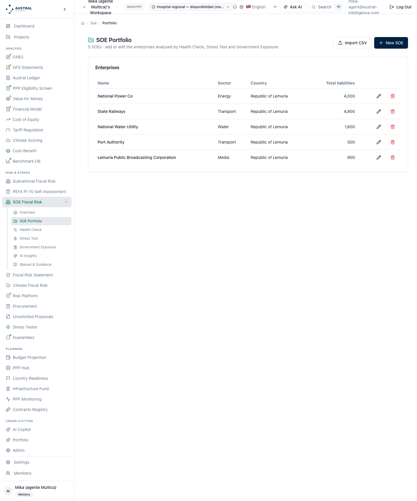
Routes: …/soe/portfolio/new and …/soe/portfolio/<enterprise>. Input: the descriptive data — name, sector, country and State ownership share, expressed as a fraction — Step 0.2's three explicit control flags, and Step 1's three blocks grouped into sections: income statement, balance sheet and transactions with government. Every field has its translated label and help note; a blank cell means not reported and produces N/A, not zero, which is exactly §3's rule. Output: the enterprise saved; calculations pick it up on the next run. Analyst decision: all of Step 1, and the Step 0.2 control test.

The form edits the full series of years, not one year. Every fiscal year is a tab, tabs are added and removed, and saving writes the whole series — so the three‑year window Step 2 needs can be built on screen for a user's own enterprise, and not only in the demonstration pack. A duplicate year is rejected with a notice. And editing a demonstration‑pack enterprise no longer wipes its series: saving now preserves the years the form did not touch, instead of replacing the whole record, so the railway keeps its 2023–2025 window and its classification does not go back to provisional. Both of these were, until recently, the module's biggest methodological gap.

The three explicit control flags — board control, golden share, contractual control — have their own three‑state selector: no evidence, yes, no. It is the route by which a 30% associate with a golden share enters the perimeter, which Step 0.2 requires and which, until recently, only the engine accepted, with no surface to declare it.

Editing carries optimistic locking: if another workspace member has changed the enterprise since the form was opened, the save is rejected with a notice inviting a reload, instead of silently overwriting.

Limits.

1. With no evidence of control and no ownership share, the entity is fully consolidated. This is Step 0.2's Austral convention — the conservative fiscal reading, declared and running against the grain of the accounting standard — and the affected entity is named in the run's warnings. Worth knowing when filling out the form: leaving all three flags at no evidence is not neutral.
2. A new enterprise with several years, loaded by CSV, needs two passes (see below). Through the form it takes one.

CSV upload — Step 1

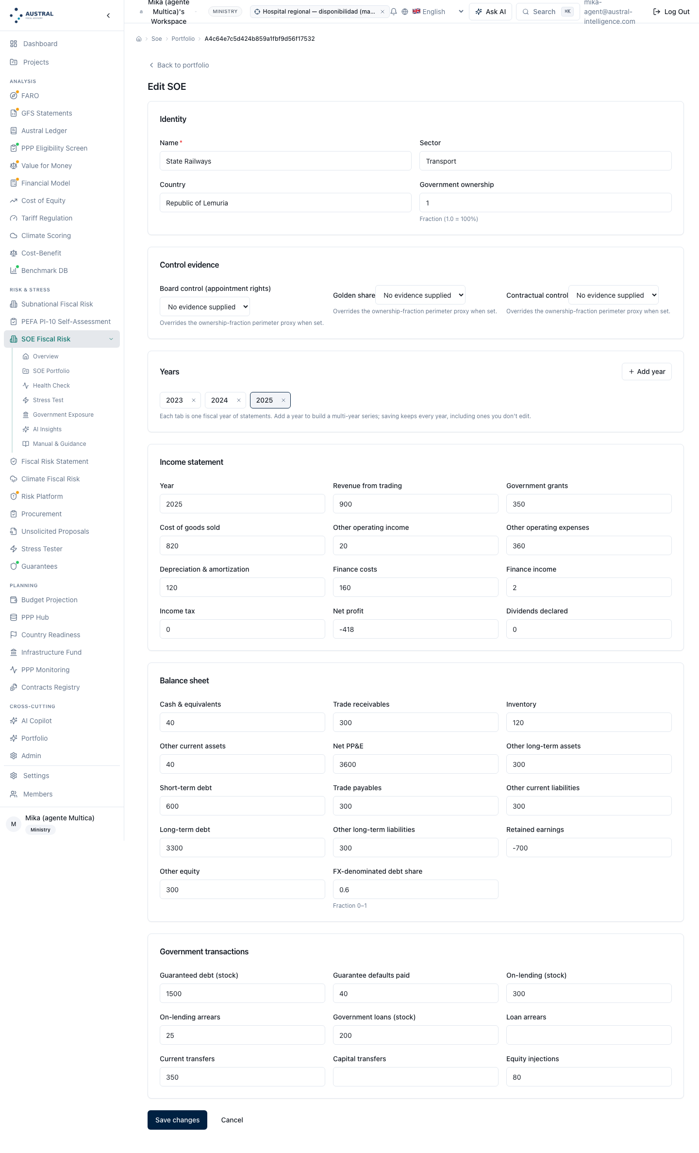
Route: …/soe/portfolio/import. Input: a CSV file whose header row names Step 1's columns. Output: the upload report — rows read, created, updated and skipped, with the error for each skipped row and warnings for unrecognized columns. Analyst decision: mapping their own spreadsheet to the method's columns.

Worth describing the contract, because it is the route by which a real portfolio comes in:

• The name column is required; a row with no name is skipped and reported.
• The id column, if it matches an existing enterprise in the workspace, updates that enterprise in place; if it does not match, it creates a new one and says so. Omitting it always creates.
• The upload accumulates by enterprise and year, which is the rule that makes the CSV route usable for a portfolio with history: each row describes one year, the one in its year cell; a year that enterprise does not yet have is added, one it already has is replaced, and every other year is left untouched. The upload never replaces an enterprise's whole series with the file's single row.
• The three explicit control flags are optional Boolean columns and are in the downloadable template.
• sector, country and ownership_pct are optional. year is an integer and, if missing, defaults to the last reference year.
• Any other column from Step 1's statement set is optional and numeric. A blank cell means "not reported" and is skipped, not turned into zero.
• A malformed cell does not break the upload: the row is skipped and reported; well‑formed rows still go in. A structurally bad file — unreadable, no data rows, no name column — is rejected in full, with the reason.
• The upload commits once, at the end of the pass, so an interrupted upload never leaves half a portfolio written.
• There is a downloadable template with the header row and two example enterprises, and it is not gated: it can be downloaded before subscribing, to learn the format.

Limits. (i) A new enterprise with several years needs two passes. The identifier is assigned by the server, so rows for an enterprise that does not exist yet cannot share an id: the first year is uploaded with the column blank, the identifier the upload report returns is read, and the remaining years are uploaded with it. That is the price of the identifier belonging to the server and not the file, and it is stated in the screen's help text. (ii) The forty‑enterprise cap applies to the enterprises created; rows that would exceed it are skipped with their reason, and updates do not count against the cap.

Health Check — Step 2 (the ratio), Step 3 and Step 4

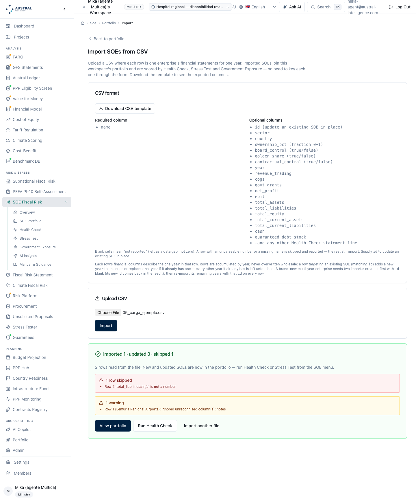
Route: …/soe/health. Input: none on screen; a button that runs the Health Check on the workspace's portfolio with the default threshold and weight set. Output: four header cards — enterprises evaluated, category distribution, list of insolvent enterprises and list of non‑market enterprises — and the enterprise‑by‑indicator heat map. Analyst decision: none on this screen; the decision is the threshold set, and today it is entered programmatically (§5.2).

The heat map carries, per enterprise: the overall rating with its category and its value to one decimal; the Z‑score with its band; the market/non‑market column, which is Step 2's binary decision with its hover note — ratio, years used and verdict; the perimeter column, which is Step 0.2's result with the ownership share in parentheses; and the fifteen category cells, each with its value and the indicator's label on hover. The insolvent enterprise carries its flag next to its name. At the foot, the note stating that the thresholds are the source's illustrative set and need country calibration.

Rows come ranked by fiscal materiality: risk category first, liabilities stock second. It is Step 4, run by the tool.

The indicator column abbreviations are readable: every indicator has its own short label, with the full label on hover, and an indicator added by a preset also gets a proper short heading instead of the automatic truncation that used to produce unreadable headers.

Limits.

1. Weighting coverage and the trend reading — what fraction of the expected weight survived the N/A indicators, and each indicator's variation over the available window with a plain‑language reading — are written and verified, and not yet integrated. When they land, coverage becomes a heat‑map and health‑sheet column in the board pack, red below 80% and amber below 100%, with the note that the rating was renormalized over the evaluable indicators, and a missing coverage is written as an empty cell and never as 0%; and the trend is read over the computable years, skips a year an insolvency guard overrode instead of interpolating it, reports not evaluable with fewer than two years, and reads direction through each indicator's sense — days receivable rising and cost recovery falling are both a worsening. The scoring ladder does not change: value, category and overall rating remain the latest year's, which is what §4 cites. [fixed, pending integration] — confirm on screen before the screenshot session.
2. While coverage is not on screen, correctly reading a rating requires looking at that enterprise's list of data gaps; and the trend across the fifteen indicators is obtained by running the Health Check year by year and comparing, or through the §5.6 route.
3. The threshold and weight set cannot be chosen from this screen (§5.2), and for the same reason §3.4's two‑axis reading has no surface: the screen publishes the overall rating with the source's weights — which is the correct axis for it — and the two relationship‑with‑government categories are on the heat map, but nothing brings them together as a second coordinate or prints the quadrant. Today the dependence axis is built by reading two heat‑map cells and the classification column. [to be built]

Stress Test — Steps 6 and 7

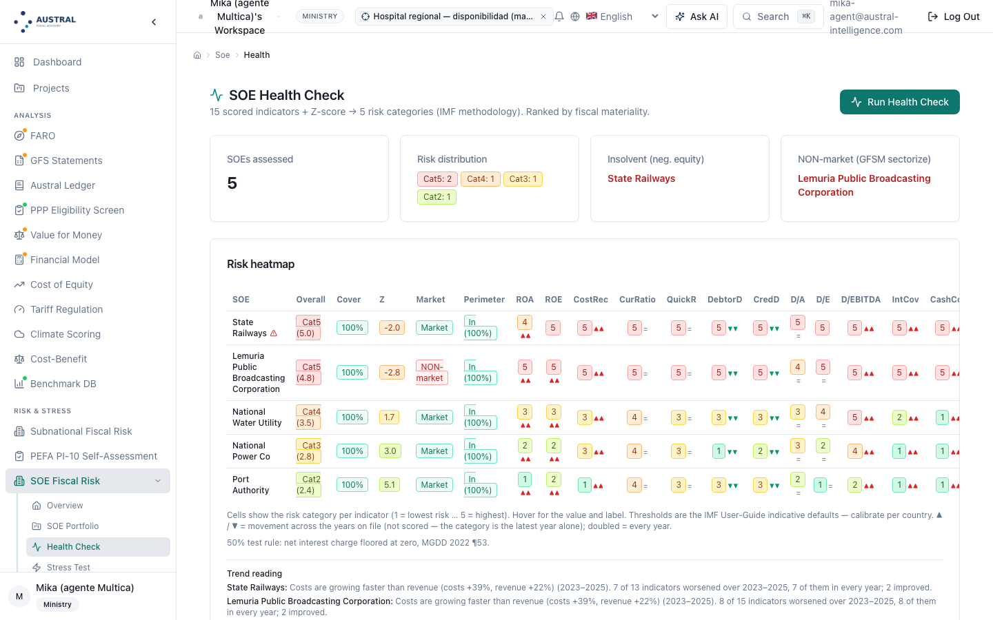
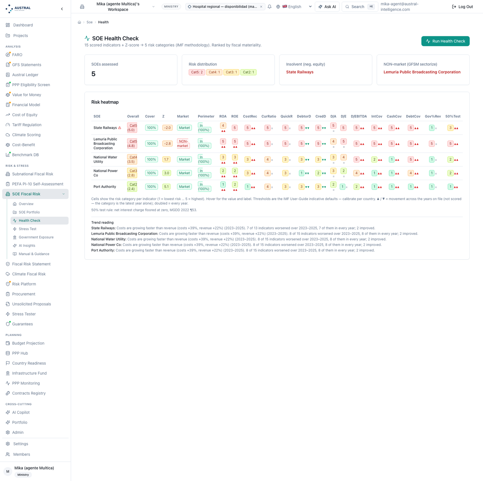
Route: …/soe/stress. Input: the scenario (mild, severe or combined), GDP for percentage calculations, GDP growth for the multi‑year path, the horizon in years, and baseline growth; two buttons, one for a single‑period stress test and one for the multi‑year projection. Output: for one period, the fiscal‑cost‑by‑channel‑and‑by‑enterprise table with a portfolio row and the total with its percentage of GDP; for the projection, the annual path as bars, the cumulative figure, and, per enterprise, the cumulative figure, the peak year, the peak year's cost, and the year‑by‑year equity trajectory. Analyst decision: the scenario, the horizon and baseline growth.

Two things this screen does today that are worth mentioning because they are recent, and because for two and a half months it showed nothing at all — the result travelled inside a three‑field envelope the client only knew how to open when it had two, and the screen failed instead of drawing its table:

1. The gross‑guarantees column is in the table, next to the incremental one, which is Step 6's rule (b) made into surface: the railway shows 0 incremental and 375 gross, and the reader sees the live exposure instead of a reassuring zero.
2. The multi‑year projection publishes its percentage of GDP, and it does so over a growing GDP path built with §4's same formula — its own GDP‑growth field, 2% by default — not over a flat GDP. The distinction is not cosmetic and is worth understanding before citing the figure: with flat GDP, Lemuria's cumulative figure comes out at 14.3%, and with the growing path, 13.5%, so the screenshot would contradict §4 if the screen used the other base. The header labels the base in full: a sum of flows over the GDP path, not a stock.

Limits.

1. The screen offers only the three preset scenarios and the sustained path. The engine additionally accepts a custom scenario — with the four magnitudes, the tax rate and the guarantee‑call fraction — and a declining path with its decay rule; neither has a control on screen. It is the limit that weighs most after §4.6's fourth reading: the declining path, which is what keeps the five‑year headline from resting on a single persistence assumption, today can only be obtained through the §5.6 route. [to be built]
2. Cost growth cannot be separated from revenue growth on screen, even though the engine allows it. It is the assumption that produces the scissors between revenue and costs, and the one that moves the projection the most.

State Exposure — Step 5

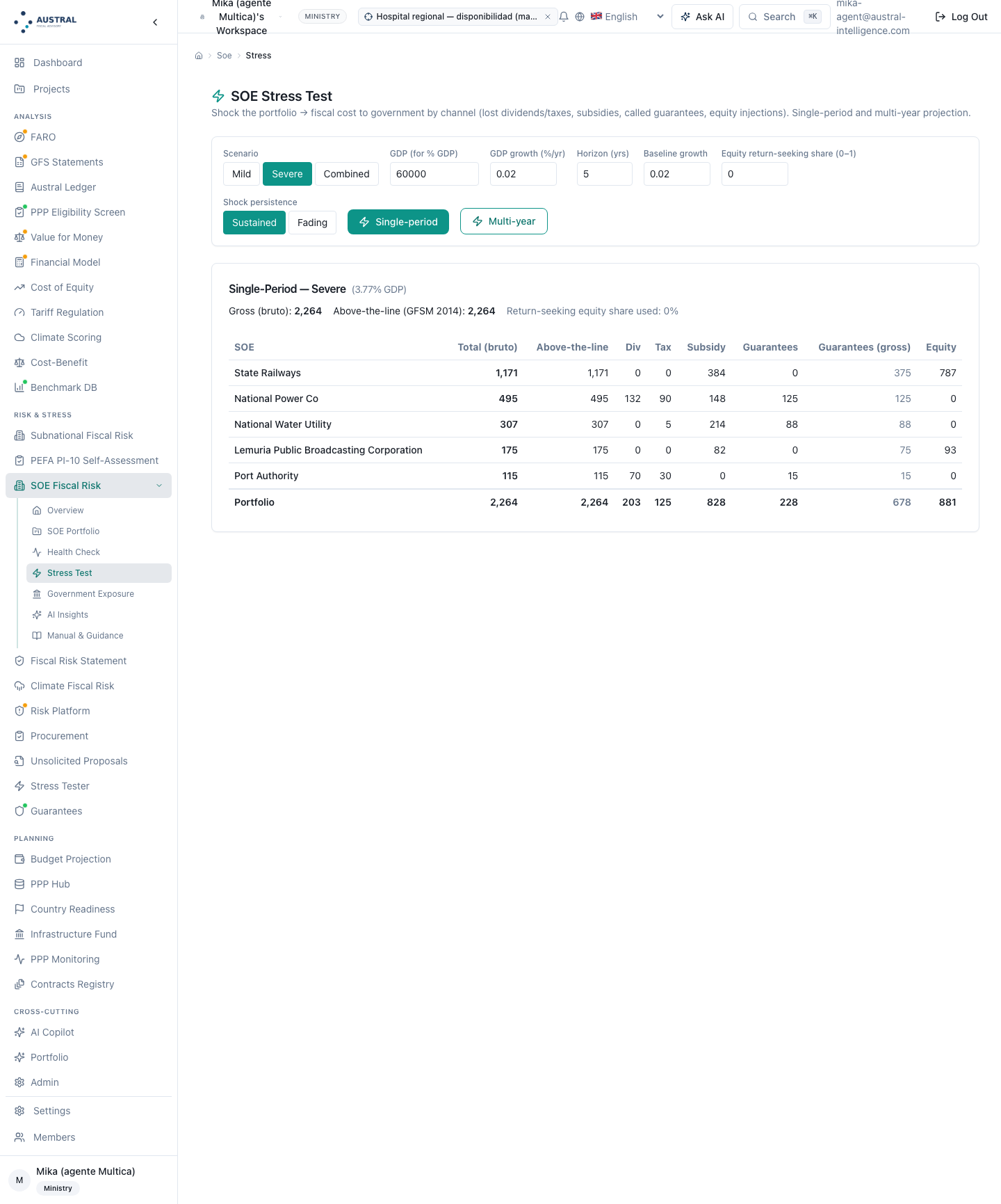
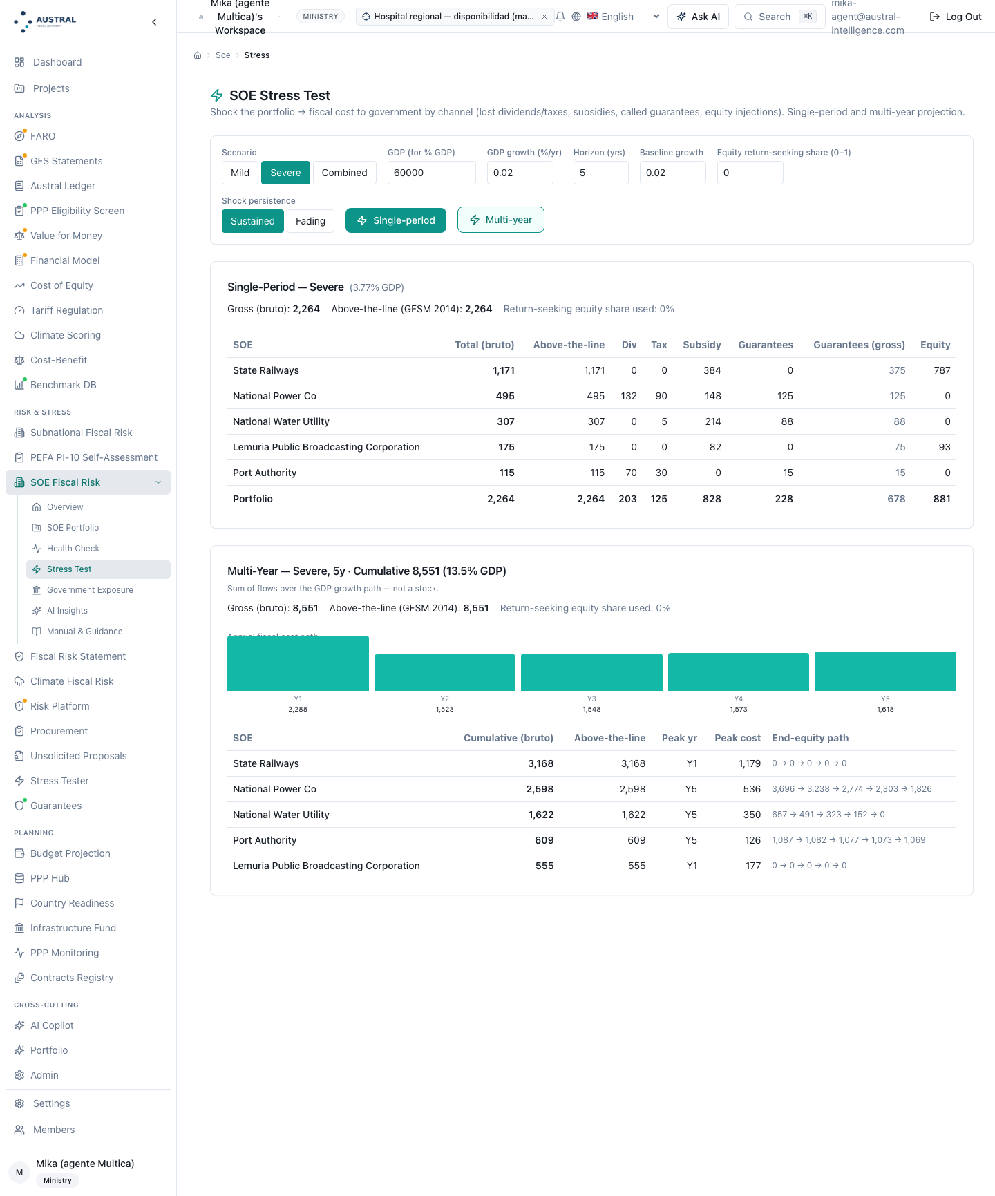
Route: …/soe/government. Input: GDP, and a calculate button. Output: four cards — contingent exposure (guarantees) with its percentage of GDP, direct claims, total exposure with its percentage, and the year's net fiscal cost — and the enterprise‑by‑enterprise table with those four figures, the materialization flag, and the warnings the engine issues: a guarantee called, with its amount, arrears on an on‑lent loan, arrears on a government loan, positive net cost, and — for the non‑market enterprise — the sectorization note with the total stock of liabilities that becomes government debt. Analyst decision: the declared GDP figure, and the reading.

The total is not the sum of the two columns, and the screen says so. For a non‑market enterprise, total exposure rises to the complete stock of liabilities — Step 5.2's rule — so the portfolio total exceeds the sum of the guarantees column plus the direct‑claims column. The total‑exposure card carries its own footnote, generated from the data itself, with the amount and the name of the enterprise producing it: in Lemuria, includes +600 from the sectorization of Lemuria Public Broadcasting. The sectorization card and the market/non‑market and perimeter flags are translated into the platform's languages, and the engine's classification note comes back already localized.

Limits.

1. The per‑enterprise warning list is still in English. The classification note the engine returns is localized, but the sentence wrapping it in the materialized‑risk card is not: in a Spanish‑language workspace, one ends up with an English sentence carrying a Spanish quotation inside it. It is the full interpretation layer, translated separately. [to be fixed]
2. The split of capital contributions has no on‑screen control. The engine accepts the fraction of contributions seeking a market return and returns, besides the net cost, the above‑the‑line cost that excludes it — which is exactly Step 5.4's convention. The screen does not offer the field and does not show that second figure: today the product always publishes the conservative convention. [to be built]
3. Exposure is calculated on the latest year. The engine knows how to produce the year‑by‑year series — which is what distinguishes chronic support from a one‑off shock — and no screen shows it. [to be built]

AI Insights — cross‑cutting

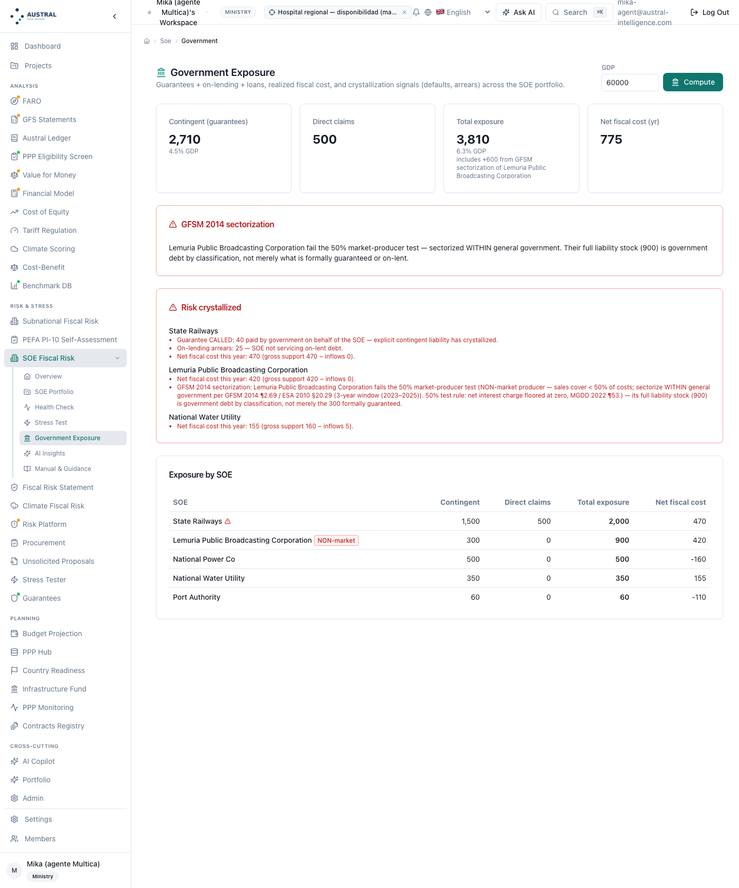
Route: …/soe/ai-insights. Input: the result of a run, and the type of text: executive summary, risk narrative or recommendations. Output: the drafted reading, with the model and the consumption declared. Analyst decision: none, other than whether to use it; the text is draft material, not a method output. It is named and shown once.

On‑screen Manual — orientation

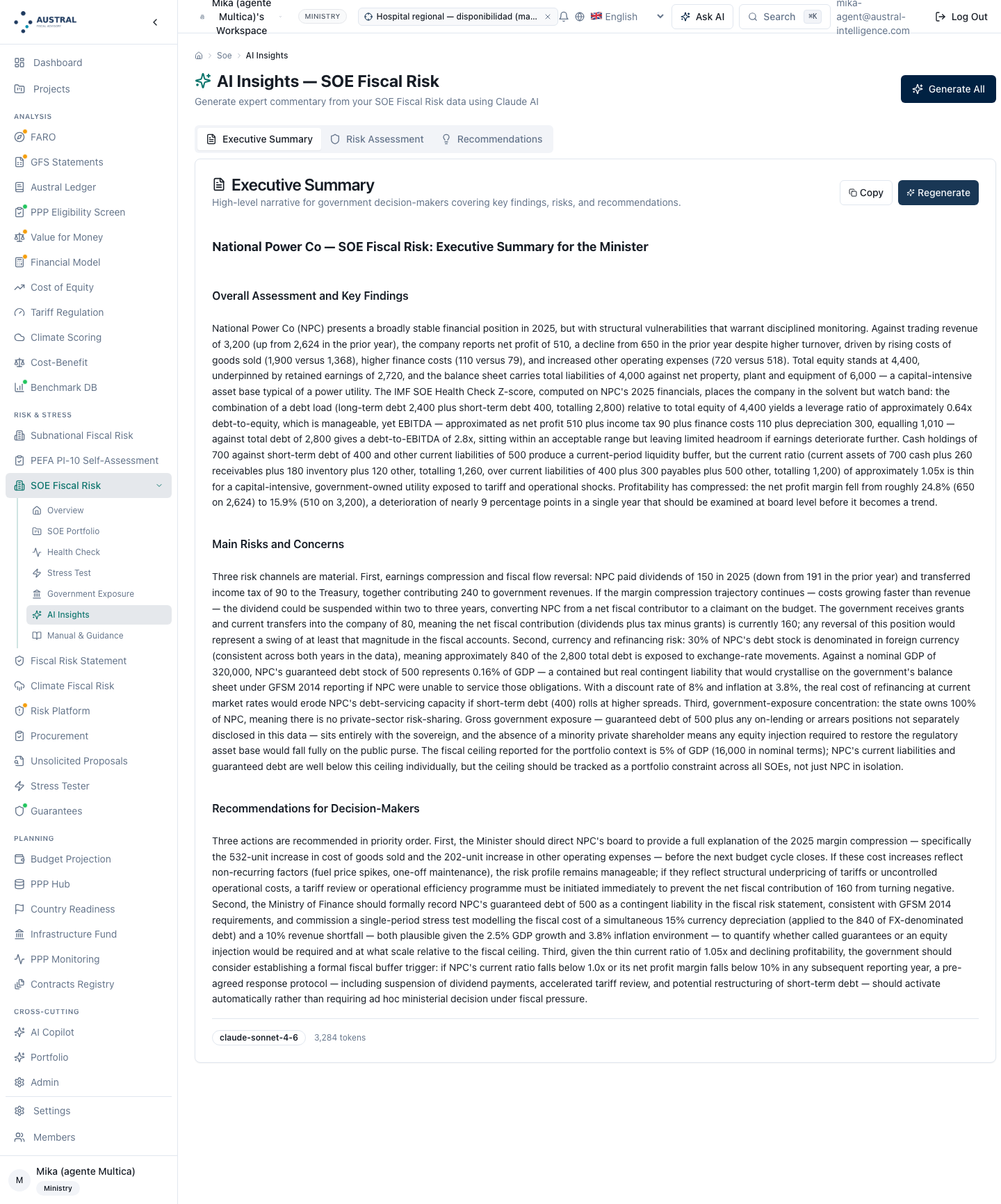
Route: …/soe/manual. Output: the method's summary within the product, in Spanish or English depending on the workspace's language, in four blocks — what it does, Health Check, Stress Test, State Exposure — plus references.

Limit. Its header already names the Austral module and credits the reference methodology as such, but the body is still out of date relative to the module it describes: it does not mention the board pack, the CSV upload, the threshold library, the interpretation layer, the market/non‑market classification or the perimeter test; and it names the 50% test without ever saying what it decides. Worth aligning with this manual now that it is written, as was done with the previous wave's modules. [to be fixed]

Board pack — Step 9 and §6 audit

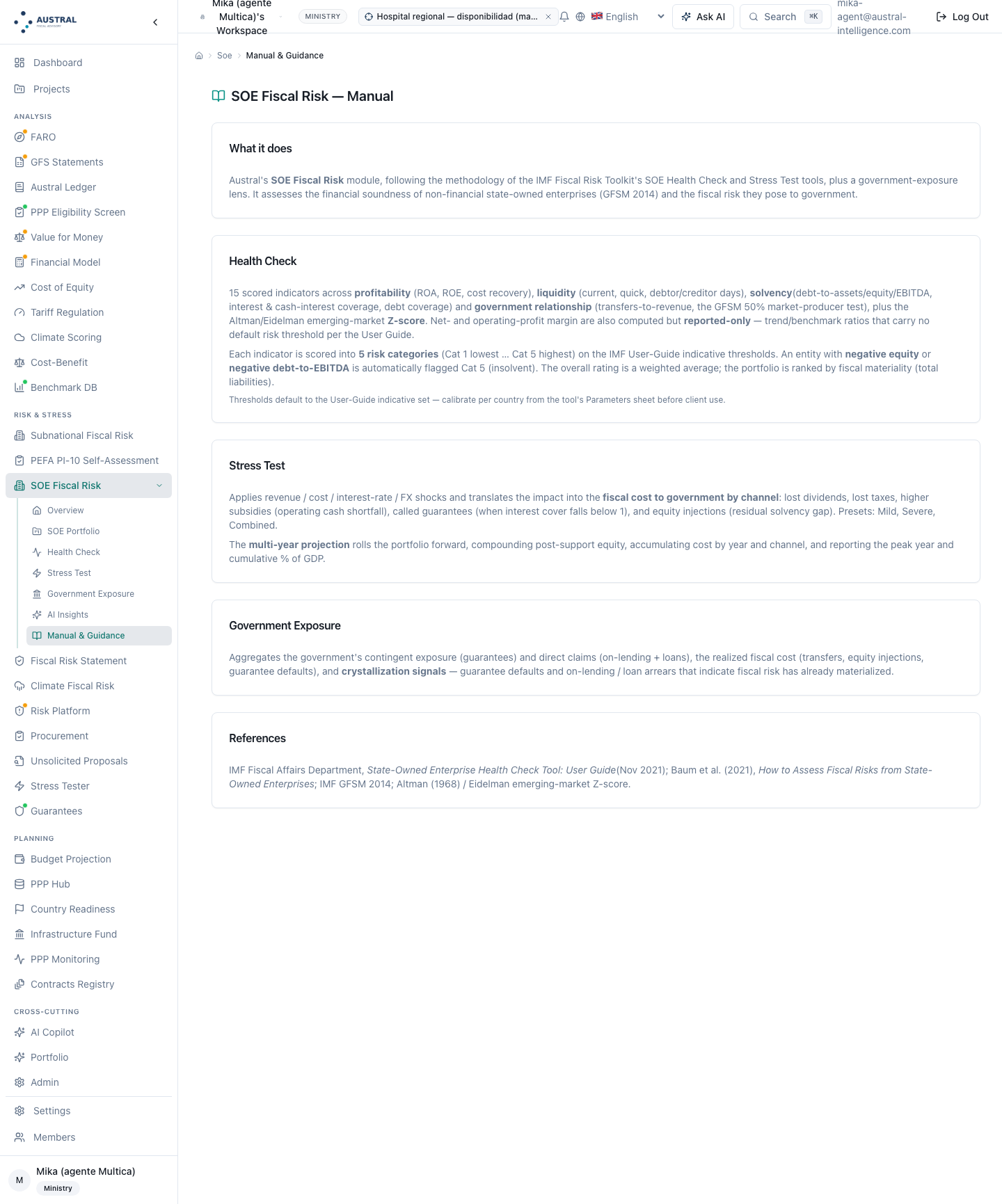
How to get it: the two buttons on the module landing page, in XLSX and PDF. Output: the same content in both formats, built from the module's own outputs with no new figures — four sheets in the workbook: (i) a cover sheet with the health verdict and its narrative, the category distribution with its colour scale, the list of insolvent enterprises, and the State‑exposure verdict with its own; (ii) health, one row per enterprise with overall category, rating, Z‑score and its band, insolvency flag and total liabilities; (iii) State exposure, one row per enterprise with total exposure, contingent exposure, direct claims, gross support, fiscal revenue, net cost and guarantee‑called flag, plus a totals row; and (iv) basis of preparation, the methodological note travelling with the document, because the pack is the copy that gets forwarded.

Limits, and these are the ones that weigh most for a ministerial deliverable.

Two things the pack already does well, worth acknowledging: the document is issued in whatever language it is asked for — sheet names, section headers, column headers and the basis‑of‑preparation note — and the totals row carries its own reclassification note, with the amount and the name of the enterprise producing it, just like the exposure screen's card. The totals figure stopped being a sum that does not reconcile without explanation.

1. It prints no percentage of GDP, even though the endpoint accepts GDP as a parameter and uses it in the calculation. The figure a minister reads first is not in the document. [to be built]
2. It does not include the stress test. The fiscal cost under scenario — §4's headline — has no sheet. [to be built]
3. It does not print the market/non‑market classification, the perimeter test or the weighting coverage, three of the outputs §3 requires to be published. Coverage arrives with the pending‑integration change; classification and perimeter, with the same one. [partly fixed, pending integration]
4. The narrative comes out in English even when the document is requested in Spanish: the labels are translated, but the interpretation layer — the cover sheet's drafted verdict — has no language parameter. [to be fixed]
5. And, as noted on the landing page, the buttons do not pass language or GDP, so today the pack always comes out in English and always without percentages even though the document knows how to do both. It is the cheapest limit to close in the whole module: two parameters on two links. [to be fixed]

IPSAS 35 Consolidation — Step 8, accounting destination

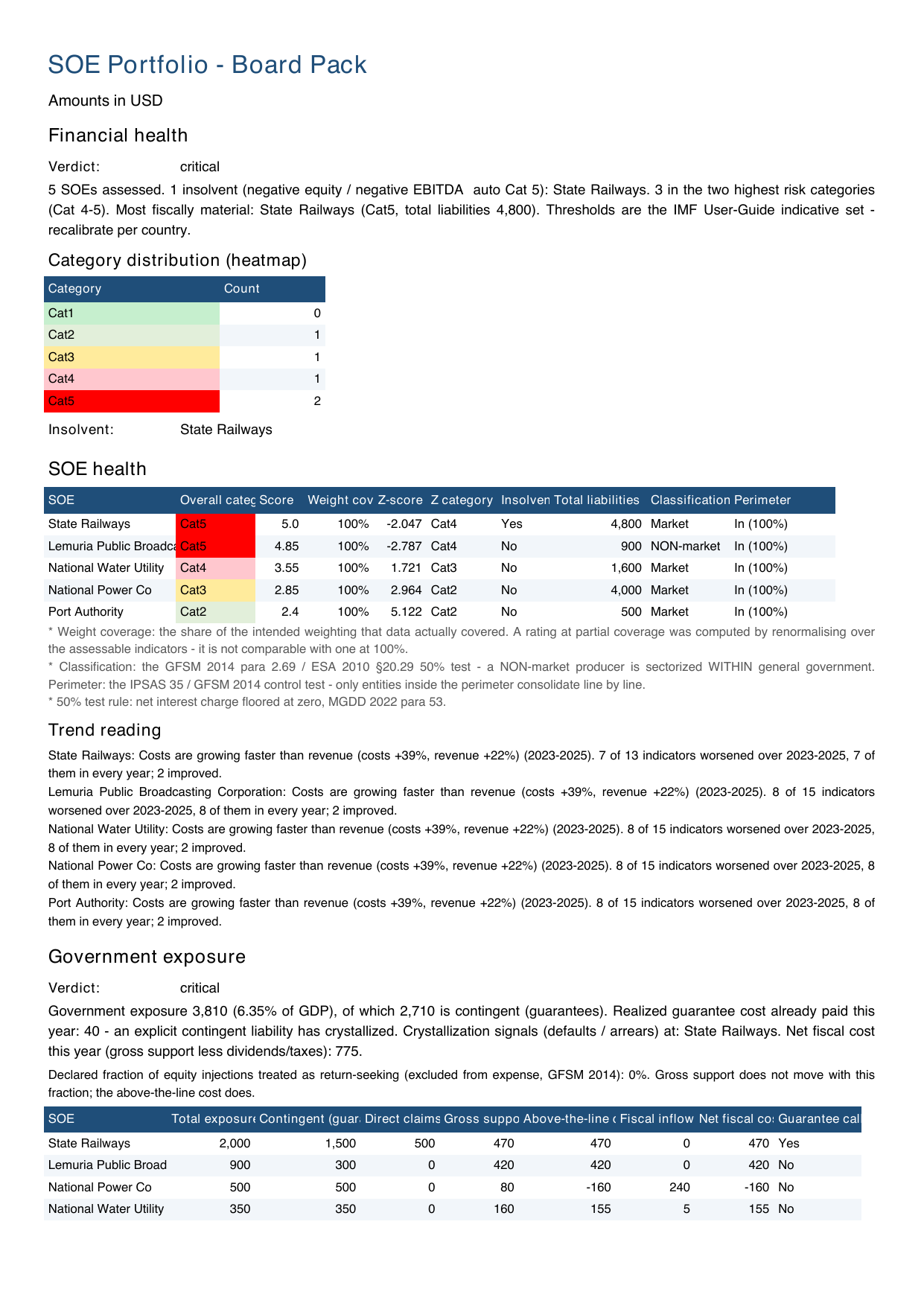
Route: …/ipsas. Consolidation reads the same portfolio of enterprises in the workspace and turns it into controlled entities, taking each one's latest year: assets, liabilities, equity, revenue, State ownership share, and the on‑lent‑loan stock as an intragroup transaction to be eliminated. It produces the consolidated statement with the non‑controlling interest and the elimination. It is shown once, as a destination, not as part of the method: whoever wants the detail goes to the accounting suite.

Limit, and its fix is already written. Consolidation today takes every enterprise in the workspace: it does not read the perimeter test's result, so an associate Step 0.2 leaves out still gets consolidated line by line, and a 30% associate with a golden share is treated under the equity method even if the Health Check screen declares it inside the perimeter. While that stands, the perimeter is controlled by deciding which enterprises live in the workspace.

The fix that closes this is written and verified, pending integration, and it is worth describing its behaviour because it changes what §5 promises. Consolidation will ask Step 0.2's test for the perimeter instead of re‑deriving it from the ownership share: inside the perimeter, it forces full consolidation; outside, it lets the standard's ladder choose between the equity method and a financial investment, instead of collapsing every associate into an investment. It also closes two silent defects worth noting on their own: a zero ownership share used to be read as 100%, and a row with the ownership share written on a percentage scale — 60 for 60% — made the enterprise disappear from consolidation with no warning, its balance sheet absent from the consolidated statement. The pack and the consolidated register will also carry the classification and the perimeter in each row's description and its provenance. No money figure moves. [fixed, pending integration] — confirm on screen before the screenshot session.

And the convention that has to be said out loud, because it is Austral's and not the standard's. When control cannot be evaluated — no declared ownership share and no explicit flag — the entity is fully consolidated and is named in the warnings of the consolidated statement. It is Step 0.2's conservative fiscal choice: it preserves the figures the register publishes today and avoids leaving out a balance sheet the State does actually own. And it deliberately runs against the grain of the consolidation standard, which requires positive evidence of control before consolidating and, in doubt, would leave the entity out. Both things are published together, with the enterprise's name in plain sight, so the reader can reverse the convention if their framework requires it. It is left flagged, not settled.

Fiscal Risk Statement — Step 8, reporting destination

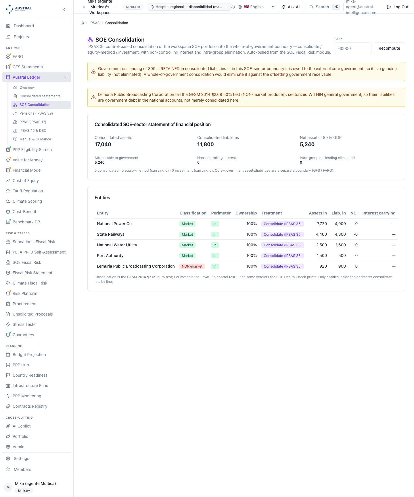
Route: …/frs. It receives the SOE portfolio as one family within the consolidated register. It is named by its route and referred to M9, its manual; it is not captured here — this §5's thirteen figures belong to the SOE module, and the fiscal risk statement has its own where it belongs.

5.2 How thresholds and weights are entered

The module publishes the source's illustrative set in its threshold library, with the four cuts for each of the fifteen indicators and their direction, and it also publishes the list of cited presets — today just one: the illustrative set itself, named explicitly and with its citation, so the selector has a baseline and so it is stated, rather than left implicit, where the default numbers come from. There are no invented country presets, and that is deliberate: the source publishes one set, and country thresholds are the analyst's calibration.

The calculation accepts a custom set: a preset by name, or the four cuts for each indicator one by one, or a complete weight set, or all three combined — explicit cuts apply on top of the preset. And it validates what it receives instead of accepting it silently: an indicator that does not exist is rejected; a ladder of cuts that is not monotonic in the indicator's direction is rejected, because it would leave a band unreachable; weights that do not sum to one, or that include a negative weight, are rejected. A badly written preset does not fall back to the default thresholds: it is rejected. The three are exactly the validations Step 3.3 requires for the result to be auditable.

But no screen offers this. Today a country calibration is loaded through the §5.6 programmatic route. It is the module's most consequential product gap after the years one: the source requires recalibration before using the tool with a client, and the product has nowhere for it. [to be built] §3.3 and §3.4 therefore describe a step the tool accepts running but does not know how to ask for.

This section describes the programmatic call instead of drawing a screen that does not exist, which is §5's rule throughout the series. And it recommends building the screen before this manual's next edition: the source requires recalibration before using the tool with a client, and a mandatory step with no surface is a step that will not get taken.

5.3 How GDP is entered

GDP is not read from the workspace's settings: it is a value typed into the screen, with a fixed starting value hard‑coded in the interface, and every screen asks for it separately. Hence a drafting rule that governs the whole of §4 and is worth making explicit:

Every "percentage of GDP" figure in this manual carries the declared GDP alongside it.

That is good practice in any case; here it is an obligation, because two screens in the same module can be using different GDP figures in the same session without saying so, and because the multi‑year projection — until fixed — does not use it at all. [to be built]: reading GDP from the workspace's settings, as other platform modules do.

5.4 What the screen says and what the engine does

Three engine conventions that §3 declares and that are worth repeating here, because they are the ones a reviewer is going to want to verify against the product:

And an invariant the analyst can check in thirty seconds, which this manual recommends running before presenting any figure: a zero‑magnitude scenario has to produce zero fiscal cost. The engine satisfies it by construction and an automated test watches over it; running it in one's own workspace is the cheapest way to confirm that what is being measured is the shock's effect and not the portfolio's structural cost.

5.5 Hand‑off to and from other modules

Today, the SOE portfolio feeds two destinations, both reading the same workspace enterprise register:

• IPSAS 35 consolidation, described above.
• The Fiscal Risk Statement, which receives it as one family within the consolidated register, with four figures per enterprise: gross exposure = total liabilities; probability, derived from the health category and raised to high if the enterprise is insolvent or its risk has materialized; realized cost = guarantees actually paid, with the year's net cost as the expected cost when it is positive; and cost under stress = Step 6's total, flagged as a deterministic scenario and not a quantile — a named scenario carries no confidence level and should not be read as if it did.

Two observations about that hand‑off, which belong in this manual because they originate here. The first: the gross exposure that travels across is the stock of liabilities, not Step 5's exposure; it is the conservative reading, consistent with Step 4, and it has to be said so no one reconciles the two figures and thinks one of them is wrong. The second: the hand‑off does not yet carry Step 2's classification or the perimeter result, so the consolidated register today does not distinguish the non‑market enterprise from the rest — precisely the enterprise whose 900 stopped being a contingency and became direct debt, and the register receives it as just another row. The fix that closes this, in the row's description and its structured provenance, is written and pending integration, and moves no money figure: it changes what the row says about itself, not what it is worth.

The no‑duplication rule with M7 and M9 is Step 8.4's, and is repeated here because this is where the reader is going to need it: the consolidated register takes the stock from this manual or the expected cost from M7, never both.

[to be built] — what does not exist today: a hand‑off to guarantee valuation (M7), to the budget, and to debt‑sustainability analysis.

5.6 Programmatic access

Everything the screens do — and several things they do not — is accessible with the account's session, on the same workspace: the portfolio's Health Check and an ad hoc enterprise's, with its calibration; the single‑period and multi‑year stress test, with a custom scenario and a declining path; State exposure, with the split of capital contributions; the threshold and preset library; creating, reading, updating and deleting enterprises; the CSV upload and its template; and the board pack's two exports, with language and GDP.

The four calls this manual needs while the screen gaps remain open are:

1. Threshold and weight calibration (§5.2): the portfolio's Health Check with a preset, with explicit cuts per indicator, or with a custom weight set — for example, the fiscal‑use set §3.4 proposes.
2. Stress test with a custom scenario and a declining path, declaring the decay rule (§5.1, the stress test's first limit). It is the route by which §4.6's two paths are obtained — and, while the screen does not offer them, the only one.
3. The multi‑year projection with the GDP path, which is today the only route to the cumulative figure as a percentage of GDP.
4. Exposure with the split of capital contributions (§5.4), which returns the above‑the‑line cost.

All four are given in prose, with their parameters named and without transcribing routes or request bodies, which is the series' external‑language convention: whoever has to run them also has the product's technical reference, and whoever reads the manual does not need an address to understand what each parameter decides.

5.7 What the module does not do, and the manual does not promise

The living list, as of this edition's close. Every entry says what the analyst does meanwhile.

And an account worth putting in writing, because it is §6's argument applied to the product itself: from the list this section carried in its previous edition, six entries came off in a single pass — the multi‑year series for a user's enterprise, the edit that used to wipe the series, the explicit control fields, GDP in the multi‑year projection, the gross figure for the guarantee channel, and the reclassified‑exposure note — and with them, the display defect that had left two of the three calculation screens showing no result at all for two and a half months. None of the six was a calculation error. All of them were surface, and surface is where a manual like this one finds them.

5.8 Step → screen map

The reverse of table 2.8.

5.9 The guest workspace, and the hand‑off

Everything described can be reproduced in the guest workspace, with no account and no cost, by loading the demonstration pack from the module's landing page: the five §4 enterprises, with the same statements and the same thresholds that produce this manual's figures. The limits declared in this section show up there just as they would in a client installation, which is why they are written down.

And the note that closes §5 in every manual in the series, which here has a precise content and not a protocol one: the client keeps the tool, and the capacity to operate it. §3's method is self‑contained and written to run without the platform; the platform exists so a team of three people can sustain the register of forty enterprises every year, with the traceability Step 9 requires, instead of rebuilding it every September. §6 explains why that difference matters more than it looks.

6. Why not in Excel, for this method

There is a concession to make first, and it is not a courtesy. The reference tool for this method is a spreadsheet, and a very good one: a spreadsheet from a public‑finance department of the International Monetary Fund, documented with its User Guide, with its input sheets, its parameters sheet and its three output sheets, able to take forty enterprises with fifteen years of history each. §3's method can be run in it. This manual is not written against that spreadsheet; it is written on top of the method that spreadsheet documents.

This section's argument is different and narrower: what happens to a spreadsheet when it stops being an instrument of analysis and becomes a register. An annual SOE register has forty entries arriving from forty different sets of books, fifteen years of history that have to be carried forward, thresholds that change when they are calibrated to the country, a reporting chain that ends in a signed budget document, and a reviewer who, three years from now, is going to ask where a figure came from. None of those four things is a calculation problem; all of them are problems of provenance, invariants and versions, and none is solved with a better formula.

The eight failures that follow are not hypothetical. Each is presented the same way: where it happens (which §3 step), what fails in the spreadsheet, how much it costs, measured on §4's Lemuria portfolio, and what the tool does instead. And several of them happened to the tool itself before being fixed; they are told that way, because the difference between a spreadsheet and a program is not that the program never gets it wrong, but that when it does, it leaves a trace and gets fixed once, for all forty enterprises.

6.1 The guarantee as the measure of risk

Where it happens. Steps 2 and 5, and it is the failure that orders all the others.

What fails in the spreadsheet. The spreadsheet sums the guaranteed‑debt column, calls it "the State's exposure to SOEs," and publishes it. It is the most natural operation in the world: the guarantee is written down, it has an amount, the State signed it. Everything else — what part of the unguaranteed debt the Treasury ends up servicing all the same — is not written down anywhere, and so has no column.

How much it costs in Lemuria. The same portfolio supports four figures, all of them true:

The first reading — the spreadsheet's — leaves out 1,100 against the third: it publishes 29% less than the exposure the method calculates, and 77% less than what the portfolio actually owes. And it does not do this because of a formula error: the sum is done correctly. It does it because a test was missing that the spreadsheet did not know it had to run.

What the tool does. Classification runs before the sum, enterprise by enterprise, and its result changes the arithmetic: for the enterprise that is not a market producer, the published exposure is its complete stock of liabilities, not the guaranteed fraction. The operation is a maximum, not a sum — it never counts the same liability twice — and it is an exact no‑op for every market‑producer enterprise, so Lemuria's four healthy enterprises carry the same figure before and after the rule. And the two readings are published with their label, because they are two questions, not one.

6.2 Revenue with transfers included

Where it happens. Step 1, at intake; it shows up in Step 2.

What fails in the spreadsheet. One cell. The revenue line on the entry form adds sales and the subsidy, because on the enterprise's income statement they sit one below the other and because in everyday conversation "what comes in to the enterprise" includes both. It is an error that produces no signal at all: total revenue comes out right, the balance sheet balances, net income does not change.

How much it costs in Lemuria. What changes is the classification of an entire enterprise. Public Broadcasting sells 160 and it costs 354 to produce:

With the cell wrongly built, the enterprise passes the test comfortably — 0.61 against a line at 2.00 — and 900 in liabilities stop being direct debt of the State, 1.5% of GDP that leaves the balance sheet because of a sum of two cells. The error is especially dangerous because it always points the same way: an enterprise financed by transfers never fails the test if transfers count as sales. The method is exactly what is meant to catch that kind of enterprise, and the cell disables it.

What the tool does. The separation is in the input form, not in the formula: transfers received are their own field in the transactions‑with‑government block, distinct from sales revenue, and no calculation in the method can confuse them because they are never in the same cell. The fix is not to warn the analyst about the formula; it is not to give them the chance to write it wrong.

6.3 Statements that do not reconcile

Where it happens. Step 1, at intake; the damage shows up in Step 6.

What fails in the spreadsheet. Net income is entered as a headline figure rather than derived from the lines above it. Someone copies it from the published financial statements, which carry extraordinary items, deferred taxes, non‑controlling interest or equity‑method results that the abbreviated entry form does not have. The entry ends up with an income figure its own lines do not produce. Nobody notices, because the entry is not used to calculate income: it is used to calculate ratios.

How much it costs in Lemuria. It happened to this portfolio. The four original entries had their net income entered as a headline, with mismatches of +210, −158, +35 and +65 against the accounting identity. The damage is not in the ratios: it is in Step 6's dividend channel, through a route nobody watches. The stress model takes the payout ratio implied by the reported income and applies it to its own recalculated income:

The payout ratio nearly doubles without a single peso of dividends changing: the State receives 150 in both worlds. Applied to the income the model recalculates, that inflated ratio destroyed more dividends than exist. The measurement recorded once this was fixed, on this same portfolio and this same scenario: 552.6 in dividends and taxes "lost," against 355 the State actually receives — a model destroying 1.56 times the available income, and contradicting the revenue figure the same system was publishing on its own exposure screen.

What the tool does. Two guards, because one alone is not enough. The accounting identity as an input validation: the entry has to satisfy net income = EBIT − finance costs + finance income − taxes, and across Lemuria's five enterprises it closes with zero residual (§4.2 table). And the two income channels capped by what the State actually receives from that enterprise‑year, which are exactly the amounts the exposure screen publishes: the severe scenario's dividend channel stops at 132 against the 150 the energy enterprise pays. The two guards make the stress model and the exposure register agree by construction and not by review.

6.4 The zero that is not a zero

Where it happens. Step 3, in any incomplete entry.

What fails in the spreadsheet. An indicator with no data gets resolved one of two ways, and both are wrong. If the empty cell is scored as zero, the enterprise's category drops because of a missing data point. If the indicator is ignored in the average, the enterprise's category rises because of a missing data point — and this is the more common one, because that is what an average function does over a range with empty cells, without saying so. The result is a rating that looks the same as the others and is not.

How much it costs in Lemuria. The water utility, with a complete balance sheet and a half‑filled income statement — no cost of sales, no other operating expenses, no depreciation:

The worse‑documented entry produces the better rating. Six of the fifteen indicators go unevaluated — cost recovery, days payable, liabilities to EBITDA and the three coverage ratios — and they are precisely the ones that gave the enterprise away: its two worst cells on §4.4's heat map disappear. A spreadsheet would publish 3.25 next to the railway's 5.00 and the port's 2.40 as if all three were comparable.

What the tool does. An indicator with no input returns an explicit N/A and is not scored. The rating is renormalized over the indicators that can be evaluated — which is the correct thing to do — and is published alongside the weighting coverage: the fraction of the expected weight that was actually used. 60% in the half‑filled entry, 100% in Lemuria's five. The number that makes ratings comparable is not the rating: it is the column next to it. A rating built on 60% of the weight is neither better nor worse than one built on 100%; it is a different thing, and the register has to say so.

6.5 Negative equity producing pretty ratios

Where it happens. Step 3, in any technically insolvent enterprise.

What fails in the spreadsheet. A division. Negative income over negative equity gives a positive number, and the spreadsheet prints it formatted as a percentage. Positive liabilities over negative equity gives a negative number, and on an indicator where lower is better, it ranks ahead of the healthiest enterprise in the portfolio. Both cells are arithmetically correct, and both are garbage.

How much it costs in Lemuria. The railway has income of −418 and equity of −400:

This is not an edge case: it is the worst enterprise in the portfolio producing, in two of fifteen indicators, the best numbers in the table. A reader scanning the heat map diagonally — which is how a heat map gets scanned — is going to see two green cells in the reddest column.

What the tool does. An entity‑level insolvency guard that does two things at once, not one. It forces the category to Cat 5 above the weighted average — an enterprise with negative equity cannot escape the highest risk category because the average of its other indicators pulls it down — and it suppresses the ratio's value, which is the part almost no one implements. Publishing +104.5% with a footnote saying "not interpretable" is trusting that no one reads quickly. The numeric rating, on the other hand, is not overwritten: the railway's 5.00 is real information about the other thirteen indicators, and flattening it to a plain 5.0 would lose data.

6.6 The guarantee cost that comes out zero

Where it happens. Step 6, in any enterprise already failing interest coverage in the baseline.

What fails in the spreadsheet. Nothing — and that is the problem. A well‑built stress model measures the incremental cost: the difference against the same enterprise's no‑shock path. That is the correct rule, and it has a consequence that has to be said out loud before publishing the table. For an enterprise that already fails in the baseline, the guarantee is called in both worlds, and the incremental channel comes out exactly zero.

How much it costs in Lemuria. It costs the report's credibility:

The two enterprises with zero incremental are the portfolio's two Cat 5s: the channel switches off exactly where the risk is greatest. And over five years the pattern widens — 1,138 incremental against 3,388 gross, three times as much. The line "zero guarantee cost for the insolvent railway" is arithmetically correct, methodologically correct, and it ends the conversation.

What the tool does. It publishes both columns together, labelled, with the explanation alongside. It does not choose for the reader, because the two answer different questions: "how much does this scenario cost me on top?" is 228; "how much do I have to pay in guarantees if this scenario happens?" is 678. And the gross figure exists in the output even when the incremental channel is zero, precisely so a live exposure does not become invisible because of a measurement convention.

6.7 The snapshot instead of the film

Where it happens. Steps 2, 3 and 7.

What fails in the spreadsheet. The spreadsheet has whichever year it has. Loading fifteen years for forty enterprises is possible, and almost no one does it, because every extra year multiplies the sheets, the formulas and the chances that a reference points at the row next door. What gets loaded is the latest close, and the method runs on it.

How much it costs in Lemuria. Three times, in three different ways.

(a) In the classification. Public Broadcasting fails the test with the three‑year window (2.09) and with its latest year (2.21). With its 2023 year — a ratio of 1.94 — it would have passed as a market producer. Which year gets picked decides whether 900 in liabilities is or is not debt of the State.

(b) In the trend. All five ratios in §4.3's table get worse every year, in all five enterprises: the railway 1.28 → 1.37 → 1.45, the energy company 0.72 → 0.82, the port 0.60 → 0.68. None is close to the line today, and all five are moving toward it at the same pace, because in all five entries costs are growing faster than revenue. That is not a fact about one enterprise: it is a fact about the portfolio, and it does not exist in any single snapshot.

(c) In the projection. The water utility has equity of 900 in 2025, Cat 4, and no materialization signal. Under the sustained severe scenario its equity runs 657 → 491 → 323 → 152 → 0, and in year five it needs recapitalization. It is the third enterprise on the priority list in the snapshot, and one of only two that are actually going to cost money in the film.

(d) In the persistence assumption, which is a film and not a data point. Even with the full series, projecting forces a choice of how long the shock lasts, and that choice moves the headline. With the same portfolio, the same initial shock and the same GDP, the five‑year cumulative figure runs from 8,551 (13.48% of GDP) if the shock is sustained to 4,489 (7.22%) if it decays linearly to zero. And it is not only the level: under the declining path the water utility never reaches zero equity — it bottoms out at 289 and recovers to 341 — so finding (c) disappears. A spreadsheet that projects does so with a persistence assumption, and almost always with just one, written down nowhere.

What the tool does. The engine accepts a path of scenarios, not a repeated scenario: the sustained and declining paths are two paths of the same shock, with the decay rule declared as a parameter, and both are published together with an identical year 1. The classification test's window is declared and multi‑year — three years when there are three — and its result says how many years it used and which ones; when there is only one, the classification is issued flagged as provisional, which is more honest than issuing it the same way regardless. The projection carries post‑support equity forward into the following year, which is what makes a chronic loss compound and a recapitalized enterprise in year 1 still costing money in year 5. And there is something the tool does not do today, which the manual states rather than hides: the Health Check scores the latest year and has no trend reading per indicator. The earlier years are loaded and the classification uses them; to see the trend across the fifteen indicators, today one has to run the Health Check year by year and compare.

6.8 Thresholds and weights with no provenance

Where it happens. Step 3.1, and it carries through to everything published afterward.

What fails in the spreadsheet. The thresholds are cells, and so are the weights. Someone put them there. In the best case they are the source's illustrative ones and nobody calibrated them to the country; in the worst case they are the source's, modified by an analyst who no longer works there, in a file with a name ending in _v3_final_revised. Forty enterprises end up scored against a parameter set no one can say where it came from, and the rating that reaches the budget document is not auditable: not because it is wrong, but because it cannot be reconstructed.

How much it costs in Lemuria. The same engine, the same portfolio, the same data, two legitimate weight sets:

Two of five enterprises change category without a single data point changing. And the choice is not exotic: the source's set leaves the two relationship‑with‑government indicators — transfers to revenue and the 50% test — at zero weight, and those are the two a finance ministry would read first. Whoever publishes a rating without publishing its weights is publishing half the number.

And there is a second wrinkle in this table that a spreadsheet has no way to give. The "fiscal‑use" set improves the water utility, from Cat 4 to Cat 3, because its problems are solvency ones and its relationship with government is spotless — and the water utility is the one that ends up at zero equity in the sustained projection. A single number does not answer the two questions the ministry is asking, and no weight set is going to fix that. The method's answer is not to recalibrate until the number looks right: it is to publish two axes — financial soundness with the source's weights, fiscal dependence as a separate coordinate — and to publish the fiscal weight set, marked as an Austral calibration, with this uncomfortable result in plain view for anyone who needs a single‑column ranking. A spreadsheet can have both columns; what it cannot guarantee is that all forty rows always get read against both, or that the weight set that produced the third column remains reconstructible three years from now.

What the tool does. The threshold set and the weight set are parameters of the calculation, not constants, and are published with the result. The only preset the tool ships with is the source's illustrative one, named and cited as such — there are no invented country calibrations — and a custom set is loaded and stays logged with the run. Where the implementation departs from the source on a single threshold, the manual attributes it to Austral by name and measures its effect (§4.4): in this portfolio it moves one indicator's category and no overall rating. A threshold that is not the cited issuer's cannot be published under that issuer's name, even when it does not move the result.

A caution against overstating the argument: today those parameters are loaded programmatically, and there is no screen that offers them, so at this point the advantage over the spreadsheet is one of traceability, not of convenience. §5.2 says so, and shows how it is done.

6.9 What is lost, and what is gained

The spreadsheet is better for understanding one enterprise. An analyst who wants to know why the water utility has a debt‑coverage ratio of 0.15 is going to learn more by opening its lines in a sheet and touching them than by reading a screen. §3's method is written so that can be done exactly that way, and §2.1's reference tool is a good place to do it.

The register is better for governing a portfolio and defending its number. The eight failures in this section have something in common, and it is not the arithmetic: none of them is a calculation error. They are a test that did not run (6.1), a badly built cell (6.2), an identity nobody validated (6.3), a gap treated as data (6.4), a valid division with no meaning (6.5), a correct convention badly communicated (6.6), one year instead of a series (6.7), and parameters with no provenance (6.8). All of them are failures of discipline sustained over time across many rows, and that is precisely the terrain where a spreadsheet — any spreadsheet, however good — loses to a system that runs the same invariants on every load, publishes the coverage next to the rating, keeps the parameter set with the run, and leaves the trail a reviewer is going to ask for three years from now.

And one last thing, which is this section's real reason for existing. Six of the eight failures above are measured with Lemuria figures because the tool itself made them at some point in its development: the income that did not reconcile, the dividend channel with no cap, the double counting of depreciation in the cost shock, the ratio value printed under negative equity, the rating with no coverage, the classification that was scored but not issued. Each was fixed once and stayed fixed for every enterprise, in every portfolio, for every client, with an automated test that keeps it from coming back. That — and not speed, or the charts, or the file size — is the argument.

Annex 6.A — Summary: failure → step → what fails → what the tool does

Every figure in this section comes from the same §4 exercise — the five‑enterprise portfolio of the Republic of Lemuria, GDP 60,000, severe scenario, five‑year horizon — and can be reproduced in the guest workspace by following annex 4.A.

7. References and further reading

All references were consulted on 23 September 2026; the Fund's two User Guides (references 1 and 2) were reread in full on 24 September 2026 against the official PDFs David downloaded that day, and their page citations come from that reading. Page convention: in the two Guides the printed page runs one unit behind the PDF viewer's page; this manual always cites the printed page. Unless stated otherwise, every document was read in its official version — a PDF downloaded from the publisher's site, or a file copy of the same PDF when the site blocks automatic download; it is stated which. ✔ = verified by direct reading for this manual · ✔M2 = verified for manual M2 in this series and not reread · ✔f = bibliographic record verified in the primary source's own reference list (reference 1), without direct reading of the document · PV = to be verified (existence confirmed; the stated fact is to be checked against the document before it is cited in the body). Where a document was read through another reference, that is stated.

Primary sources for the manual

1. International Monetary Fund (2021). State Owned Enterprise Health Check Tool: User Guide. Fiscal Risk Toolkit series. Washington, D.C., November 2021, 35 pp. Title: exactly this, with no hyphen in "State Owned," as printed on the cover; the header on p. 3 reads State‑Owned Enterprise Health Check Tool User Guide, hyphenated and without a colon. This manual cites the cover version. Authorship: the cover reads "Prepared by Avril Halstead, Chris Marrison, Patrick Ryan, and Amanda Sayegh"; note 1 (p. 3) specifies the division of labour — the tool was prepared by Avril Halstead, Patrick Ryan and Amanda Sayegh, "with substantial inputs from Chris Marrison and Kezhou Miao" — and thanks eleven other Fund staff for comments. It carries no series number or DOI. Cited by section and printed page (one less than the viewer's): §I, pp. 3‑5 (purpose, scope, the five fiscal‑risk channels, the historical scale of support, the disclosure warning); §II, pp. 5‑6, and table 1, p. 6 (fiscal risk ↔ financial indicator, and the narrative list of indicators by family); §III, pp. 6‑7, and figure 1, p. 7 (structure and workflow); §IV.A, pp. 7‑8 (inputs, caps of 40 enterprises and 15 years, five categories, the automatic Cat 5 flag on the indicator, common thresholds) and §IV.B, p. 8 (indicator selection and weighting); §V.A, pp. 9‑10 (scope: non‑financial public corporations; does not project; same thresholds across the sector) and §V.B, pp. 10‑11 (two‑stage process; liabilities as a proxy for exposure; table 2); §VI, p. 12 (references); annex I, p. 13 (structure); annex II.A, p. 14; annex II.B, pp. 15‑20 and table A2.1, pp. 18‑20 (the definition of every input line, including guarantees, on‑lent loans, arrears, capital transfers and capital contributions); annex II.C, pp. 21‑28, with figure A2.4, p. 21 (formulas for the seventeen calculated indicators and the Z‑score), figure A2.5, p. 22 (illustrative threshold set, in four blocks and fifteen scored indicators plus the Z‑score), the threshold reasoning, pp. 22‑25, note 6, pp. 24‑25 (simplifications in the 50% test and the window warning), box 1, p. 25 (Z‑score), tables A2.2, p. 26 and A2.3, p. 27 (Merton and rating‑average approaches), and the regression approach, pp. 27‑28; annex II.D, p. 28 and figure A2.6, p. 28 (indicator selection and weights: thirteen boxes, without the two relationship‑with‑government ones); annex II.E, pp. 29‑30; annex II.F, pp. 30‑31; annex III, pp. 32‑34 (interpretation guide, with each indicator's formula). ✔ (official PDF, local copy downloaded by David on 24‑09‑2026; figures A2.4, A2.5 and A2.6 were read rendered from the PDF itself, because they are images and not text, and the §5 engine's default set was checked against them threshold by threshold and weight by weight). This is one of the two sources whose documented method the §5 module reimplements (D12); its files are not reproduced, and its name is not used as a product name (P14). A reading note, for anyone following the citations: the Guide has four misdirected internal cross‑references worth knowing about — §IV (p. 7) points to "Annex I" for step‑by‑step instructions, which are actually in annex II; §IV.B (p. 8) points to "Annex II" for indicator interpretation, which is actually in annex III; §III (p. 6) mentions "Figure 2" for the workflow, which is labelled figure 1; and annex II.C (p. 21) points to a "Table A2.4" that does not exist in the document, whose content is in annex III and in the Ratio Metadata sheet. This manual's citations use the real location. Two further internal discrepancies, discussed in §2.1 because they affect what is published: §II (p. 6) names a profitability indicator — "return on working capital" — that appears in neither figure A2.4 nor figure A2.5 nor annex III; and the reasoning behind the return‑on‑equity thresholds (p. 22) uses 15% and 8%, while figure A2.5 on the same page prints 0.20 and 0.10.
2. International Monetary Fund (2022). State‑Owned Enterprises Stress Test Tool: User Guide. Fiscal Risk Toolkit series. Washington, D.C., May 2022, 81 pp. Prepared by Anja Baum, Alberto Soler and Mouhamadou Sy (cover). On the date, because the file is misleading: the local copy was saved as ..._Jan2023.pdf and the source inventory catalogued it as "January 2023," but the document's cover reads May 2022, and the PDF carries no title, author or authorship‑date metadata to support otherwise (its file‑creation date, January 2024, belongs to a later regeneration, not the publication). This manual cites May 2022; if David has the January 2023 reference from the publisher's page, that is the site's publication date, and it must be stated which one is used. Cited by section and printed page, which in this Guide matches the viewer's (unlike reference 1): §I, pp. 5‑9 (objectives; two modules — peer comparison and stress test; six‑year horizon; baseline and stress scenarios; sheet structure and table 1); §II to §IV.7, pp. 10‑29 (inputs and assumptions; §IV.4, p. 24, the fraction of the capital contribution expected to be remunerated at market prices, recommended at zero out of prudence; note 9, p. 23, calibration references for the liquidity floor and the leverage ceiling); §IV.8, pp. 30‑34 (catalogue of macroeconomic and market shocks; additive and multiplicative shocks; note 22, p. 33, calibration by standard deviation and the 10‑15% threshold as a "very large" shock; note 23, pp. 33‑34, the scenario narrative); §V, p. 35 (peer comparison on the ORBIS base, around 22,000 comparables, around 83 sectors, NACE classification and income‑level grouping); §VI to §VII, pp. 36‑59 (projection of debt and the three statements); §VIII, pp. 60‑66 (financing and bailout decisions: the capital contribution as the realization of an implicit contingent liability, the cash → debt → contribution order, the deliberate exclusion of arrears and overdrafts in note 43, p. 61, and the no‑bailout counterfactual); §IX, pp. 67‑71 (statements in government‑finance‑statistics terms, with tables 25 and 27 mapping to GFSM 2014); §X, pp. 72‑74 (relations with government: budget revenue and expense, net flows with and without transfers, equity, loan and guarantee stocks, and intertemporal aggregation in present value, notes 53 and 54, p. 74); §XI, pp. 75‑78 (performance indicators, with reference thresholds: interest coverage below 1.2, quick ratio below 0.8, liabilities to equity above 1.5, liabilities to assets above 0.75, non‑current liabilities to assets above 0.5); §XII, p. 79 (charts). Its note 1 (p. 5) credits reference 3 and Baum et al. (2020), Managing Fiscal Risks from State‑Owned Enterprises, IMF WP 2020/213, as its methodological sources. ✔ (official PDF, local copy downloaded by David on 24‑09‑2026, read directly for this manual). It is the second of the two §2 sources; Steps 6 and 7 of §3 declare their four departures from it.
3. Baum, A., Medas, P. A., Soler, A. & Sy, M. (2021). How to Assess Fiscal Risks from State‑Owned Enterprises: Benchmarking and Stress Testing. IMF How To Notes 21/09 (also catalogued by the publisher as 2021/009), Fiscal Affairs Department, Washington, D.C., August 2021. The framework for the SOE stress test and peer comparison; the diagnose → stress → fiscal‑cost chain. ✔f title and authorship (reference 1, §VI, p. 12; also cited in §I, p. 3 and §V.B, p. 11) · ✔ series number and date, now through two independent routes: the publisher's catalogue and reference 2's note 1 (p. 5), which gives the number "21/09" and the publisher's link dated 18‑08‑2021 · PV direct reading and chapters: the Fund's site returns 403 to automated download from this environment, and this was not worked around. (Closes R2 from the index, except for the chapters. §2.2 no longer depends on this note to describe the stress test: that description now comes from reference 2, read directly.)
4. International Monetary Fund. Fiscal Risk Toolkit. The family the Health Check belongs to: the PPP fiscal risk assessment model (PFRAM), the fiscal risk assessment tool, the public sector balance sheet assessment, the SOE health check and stress test, the fiscal stress test, the COVID‑19 stress test, and the standardized guarantee and discrete guarantee/loan tools. ✔ the list of nine tools and their acronyms, read on the cover diagram of references 1 and 2, which print it identically eleven months apart; the acronyms are PFRAM, FRAT, PSBS, SOE‑HCT, SOE‑ST, FST, C‑ST, SGAT and DGAT (the last, Discrete Guarantee and Loan Assessment Tool) · PV the publisher's currently published list.
5. International Monetary Fund (2014). Government Finance Statistics Manual 2014. Washington, D.C. Ch. 2: ¶¶2.42‑2.45 (artificial subsidiary, central borrowing authority, ancillary activity); ¶¶2.64‑2.75 (market and non‑market producer; ¶2.66 economically significant prices; ¶2.69 half of costs over a sustained multiyear period; ¶2.70 and note 22 case by case, range of years and hysteresis; ¶2.71 support and guarantees tilt toward non‑market; ¶2.72 a captive supplier; ¶2.73 sales; ¶2.74 production costs with a return to capital); ¶¶2.104‑2.106 (why public‑corporation statistics are compiled; ¶2.105 reclassification in both directions); ¶¶2.107‑2.112 and box 2.2 (control: the eight indicators); ¶¶2.113‑2.123 (types of public corporation, public‑sector aggregates); figure 2.4 and ¶2.124 (decision tree); figures 2.2 and 2.3. Ch. 7: ¶¶7.251‑7.256 and note 74 (explicit and implicit contingent liabilities; 6M61‑6M63; nominal‑value memorandum item; "assuming unguaranteed debt of public sector units" as an implicit contingency). https://www.imf.org/external/Pubs/FT/GFS/Manual/2014/gfsfinal.pdf. ✔ (official PDF downloaded and read). (Closes R3 from the index on the GFSM side.)
6. European Union (2013). European System of Accounts — ESA 2010 (EU Regulation No. 549/2013). Luxembourg: Publications Office of the European Union. Ch. 20: §§20.17‑20.18 (control); §§20.19‑20.28 (economically significant prices and buyer criteria); §20.29 (the four qualitative conditions and the 50% criterion); §20.30 (sales) and §20.31 (production costs, with the net interest charge); §§20.32‑20.34 (financial intermediation); §§20.35‑20.37 (public groups; the test applies to the individual unit). https://ec.europa.eu/eurostat/documents/3859598/5925693/KS‑02‑13‑269‑EN.PDF. ✔ (official PDF downloaded and read).
7. Eurostat (2023). Manual on Government Deficit and Debt — Implementation of ESA 2010, 2022 edition. Luxembourg: Publications Office of the European Union (KS‑GQ‑23‑002), February 2023. Ch. 1, §1.2.4.2 (specific producer cases, ¶¶49‑50) and §1.2.4.3 "The quantitative market/non‑market test" (¶¶51‑57: ¶52 what is and is not a sale, with the per‑ticket‑subsidy‑versus‑lump‑sum example; ¶53 production costs and the net interest charge, with its zero floor; ¶54 priority of the qualitative criteria; ¶55 a window of at least three years, applied at the individual institutional‑unit level, hysteresis; ¶56 quasi‑corporations; ¶57 new enterprises); §1.2.4.4 (units in liquidation). https://ec.europa.eu/eurostat/web/products‑manuals‑and‑guidelines/w/ks‑gq‑23‑002. ✔ (official PDF downloaded and read). (Closes R3 on the European side.)
8. IPSASB. IPSAS 35 — Consolidated Financial Statements. New York: IFAC; 2025 edition Handbook text. ¶¶1‑5 (objective and scope; ¶4 refers to IPSAS 40); ¶14 (definitions: control, power, benefits, binding arrangement, non‑controlling interest, relevant activities, protective rights); ¶¶18‑22 (the principle and its three elements); ¶¶23‑29 (power; ¶24 rights other than voting rights; ¶25 statutory autonomy; ¶26 regulation and economic dependence are not enough; ¶29 protective rights); ¶¶30‑34 (variable benefits); ¶¶35‑37 (the link between power and benefits); ¶¶38‑42 (consolidation procedures; ¶40(c) full elimination of intragroup transactions); ¶¶47‑50 (non‑controlling interest); AG12 and AG41‑AG42. https://ifacweb.blob.core.windows.net/publicfiles/2025‑04/B08_IPSAS_35.pdf. ✔
9. IPSASB. IPSAS 40 — Public Sector Combinations. New York: IFAC; 2025 edition Handbook text. ¶¶1‑2 (objective), ¶¶3‑4 (scope), ¶5 (definitions of amalgamation, acquisition, combined entity and acquirer) and ¶¶6‑8 (classifying the combination by who obtains control). ✔ objective, scope, definitions and classification · PV the recognition and measurement paragraphs, which this manual does not use. 9bis. IPSASB. Handbook of International Public Sector Accounting Pronouncements, official Spanish translation, 2022 edition, three volumes. New York: IFAC. In the Spanish edition of this manual, this was the source of the official Spanish form of the §2.4 consolidation terms and of the AG↔GA paragraph‑numbering equivalence declared there. This English edition quotes the English Handbook directly, so no such equivalence needs to be declared here; the entry is kept for provenance, since it is the source that fixed those Spanish‑language decisions in the manual's Spanish edition. Vol. 2: IPSAS 35 ¶14 (definitions, p. 388) and its application guidance AG12 (p. 400) and AG41‑AG42 (p. 405), numbered GA in the official translation, with the same numbers and the same content in English. ✔ (read in the volume, at the pages cited). The three volumes are copy‑protected: terms and short passages are cited, and the text is not reproduced, nor is it in the repository.
10. System of National Accounts 2008, institutional‑sectorization chapter. Withdrawn from the index: §2.3 was resolved with GFSM 2014 and ESA 2010, which are the sources the tool and the module cite, and adding the SNA 2008 would have been a third drafting of the same rule with no consequence for the method.

SOE fiscal risk and corporate governance

1. International Monetary Fund (2016). Analyzing and Managing Fiscal Risks — Best Practices. IMF Policy Paper, Washington, D.C., June 2016. SOEs on the fiscal‑risk map; "Fiscal Risk Analysis and Management," §C (fiscal stress test). ✔M2 (file copy).
2. International Monetary Fund (2019). Fiscal Transparency Code, pillar III (fiscal risk analysis and management). ✔M2. Companion: International Monetary Fund (2018), Fiscal Transparency Handbook — reference 1 cites it alongside the Code as the disclosure guide for SOE contingent liabilities, quasi‑fiscal activities and transactions with government. PV principles to be cited.
3. International Monetary Fund (2020). Fiscal Monitor, April 2020, chapter 3, "State‑Owned Enterprises: The Other Government." The source of the magnitudes reference 1 cites in its §I (the world's largest SOEs' assets equal to about half of world GDP in 2018; their debt; their weight among the world's two thousand largest companies). ✔ edition, chapter and title · PV direct reading and pages.
4. OECD (2024). Guidelines on Corporate Governance of State‑Owned Enterprises. Paris: OECD Publishing. Revised edition adopted by the Council at ministerial level in May 2024 and launched in October 2024, with a new chapter on SOEs and sustainability. ✔ edition and date · PV chapters to be cited. Corrects the index, which left it as the "current edition": reference 1, from 2021, necessarily cites the previous edition, so citing the Guide and the Guidelines together requires stating which edition each one uses. Companion: OECD (2024), Ownership and Governance of State‑Owned Enterprises, with comparative data across 59 jurisdictions. PV.
5. World Bank (2014). Corporate Governance of State‑Owned Enterprises: A Toolkit. Washington, D.C.: International Bank for Reconstruction and Development / World Bank. ✔f (reference 1, §VI) · PV direct reading and chapters.
6. Bova, E., Ruiz‑Arranz, M., Toscani, F. & Ture, H. E. (2016). "The Fiscal Costs of Contingent Liabilities: A New Dataset." IMF Working Paper 16/14. Washington, D.C. The source of the historical average of 3% of GDP — and the maximum of 15% — of support to individual SOEs cited in §2.2. ✔f authorship and working‑paper number (reference 1, §VI) · PV direct reading. Corrects the index on the fourth author's initial (H. E. Ture) and fixes the number.
7. Allen, R. & Alves, M. (2016). "How to Improve the Financial Oversight of Public Corporations." IMF How To Notes, Washington, D.C. ✔f title and authorship (reference 1, §VI) · PV series number and direct reading. Further reading on portfolio financial oversight, which this manual does not cover and which is a governance matter.
8. Polackova Brixi, H. & Schick, A. (eds.) (2002). Government at Risk: Contingent Liabilities and Fiscal Risk. Washington, D.C.: World Bank / Oxford University Press. ✔M2 title · PV chapters.
9. Scott, D. (2007). Strengthening the Governance and Performance of State‑Owned Financial Institutions. Policy Research Working Paper 4321. Washington, D.C.: World Bank. Entry‑level reading on financial SOEs, which this method excludes (§2.1). ✔f (reference 1, §VI) · PV direct reading.

The Z‑score and where it comes from

1. Altman, E. I. (1968). "Financial Ratios, Discriminant Analysis and the Prediction of Corporate Bankruptcy." The Journal of Finance, September 1968, XXIII(4), pp. 589‑609. ✔f full record (reference 1, §VI) · PV direct reading.
2. Altman, E. I. (2005). "An Emerging Market Credit Scoring System for Corporate Bonds." Emerging Markets Review, 6, pp. 311‑323. The emerging‑markets variant, with the constant 3.25. ✔f full record (reference 1, §VI and box 1) · PV direct reading. Corrects the index, which attributed the emerging‑markets variant to Altman, Hartzell and Peck (1995/1998): the primary source cites this work, and dates the model's development to 1993.
3. Eidelman, G. J. (1995). "Z scores — A Guide to Failure Prediction." CPA Journal, February 1995, 65(2), pp. 52‑54. The constant‑free variant — the one the tool and the module apply — and its bands of 2.6 and 1.1. ✔f full record (reference 1, §VI and box 1) · PV direct reading.

Country practice

1. Chile — Budget Directorate, Ministry of Finance (2025). Informe de Pasivos Contingentes 2025 (Contingent Liabilities Report 2025). Santiago, December 2025. Ch. I.2.2 (risk factors of the State guarantee to SOE debt); tables 2 and 3 (contingent‑liabilities summary as % of GDP, with the SOE guarantee reported as maximum exposure); ch. III.3 (the twelve laws with guaranteed debt outstanding as of 30 September 2025; the constitutional and Decree Law 1.263 requirement of authorization by law; the share of State enterprises' gross debt that is guaranteed); table 22; ch. VI (residual value of port and water‑utility enterprises). https://www.dipres.gob.cl/598/articles‑400549_doc_pdf.pdf. ✔ The structure, the method and the published aggregate magnitudes are cited; no enterprises are named and no client figures are used.
2. Chile — Ministry of Finance. Informe de Estadísticas de la Deuda Pública (Public Debt Statistics Report) (December 2025 edition, data as of September 2025). Gross debt of SOEs and State‑guaranteed debt. PV: the ministry's site blocks automated download from this environment, and the document was not read. §2.7 does not use this report: it derives the order of magnitude of SOEs' gross debt from the two figures reference 23 does publish — maximum exposure as % of GDP and the guaranteed fraction of gross debt. If David wants to cite it directly, the PDF has to be opened by hand.
3. Chile — Decree Law No. 1.263 of 1975, Organic Law on State Financial Administration, art. 40, fifth to seventh paragraphs, added by art. 18 of Law No. 20.128 on fiscal responsibility (2006): the annual obligation to report State guarantees and contingent liabilities. ✔M2 (text read in both norms for that manual). The State Enterprise System as State owner: PV norms to be cited; not used in the body.
4. Peru — Law No. 27170, Law of the National Fund for Financing State Business Activity (FONAFE). A public‑law legal entity under the Economy sector, responsible for setting rules for and directing State business activity. ✔ existence and purpose (text of the law in the Congress repository) · PV articles to be cited, current regulations, and the Ministry of Economy and Finance's report on the portfolio.
5. Colombia — State industrial and commercial enterprises within the Medium‑Term Fiscal Framework. PV in full: the norm requiring the report, the chapter, the periodicity and exactly what is published per enterprise were not verified. Table 2.6's row is written at the level of generality that verification allows, and must be checked before publication.
6. South Africa — National Treasury (2026). Budget Review 2026, chapter 7, "Government Debt and Contingent Liabilities," section "Contingent liabilities" (defining guaranteed amount versus exposure) and table 7.10 "Government guarantee exposure," with entity‑level detail in table 11 of the statistical annex. https://www.treasury.gov.za/documents/National%20Budget/2026/review/Chapter%207.pdf. ✔ (official PDF downloaded and read). The disclosure structure and the definition are cited; its figures are not used.
7. United Kingdom — HM Treasury. Whole of Government Accounts. Consolidation of government‑controlled entities under accounting criteria. ✔M2 (edition for the year ended 31 March 2023, HC 289, November 2024) · PV the edition current as of M6's publication.

Austral papers

Cited as "Austral, title." All are published at https://austral‑intelligence.com/research/ (Spanish version at https://austral‑intelligence.com/es/research/), with HTML and PDF at the same address. Series numbers are omitted, as in M2, pending unification of each paper's header with the site's index.

1. Austral (2026). The Anchor and the Perimeter. §3.2 (the market‑producer test applied entity by entity to Chile's twenty‑eight State enterprises over cumulative 2017‑2024 results, with its decision rule and results table); §3.1 (the firm concession commitment as omitted debt); §3.3 (the gap and its evolution); §3.4 (the anchor's perimeter in international context). https://austral‑intelligence.com/research/chile‑augmented‑debt/. ✔ (read for this manual). Launched 24 September 2026 (D9); the manual cites it as published.
2. Austral (2026). The Recognition Rule — When a PPP Lands on the Government Balance Sheet (and How the Line Is Gamed). §4 (where the rulebooks diverge), §6 (the recognition gap). SSRN 7383122. https://austral‑intelligence.com/research/recognition‑rule/. ✔M2
3. Austral (2026). The Useful Silence — Why Governments Choose the Liability They Cannot See. §2 (the mechanism), §7 (reform ranking). SSRN 7389838; DOI 10.2139/ssrn.7389838. https://austral‑intelligence.com/research/useful‑silence/. ✔M2
4. Austral (2026). Stress‑Testing PPP Portfolios — Macro Shocks at Programme Level. §2 (why a common stress does not diversify away), §4 (correlation structure), §5 (shock catalogue). https://austral‑intelligence.com/research/stress‑testing‑portfolios/. ✔M2 Cited for the correlated‑portfolio logic, carried over here from a portfolio of contracts to one of enterprises.
5. Austral (2026). The Optimal Risk‑Retention Frontier — How Much Risk a Ministry of Finance Should Keep. §2 (the frontier), §5 (retention as a contingent liability). https://austral‑intelligence.com/research/retention‑frontier/. ✔M2
6. Austral (2026). Foundations for Deciding When to Use a Third‑Party Guarantee. §11 (limits: does not model call probability). https://austral‑intelligence.com/research/third‑party‑guarantee‑decision/. ✔M2 This is the frontier with M7: this manual records the SOE's guarantee at face value and does not price it.
7. Austral (2026). The Pipeline Under the Ceiling. §§2‑3 (headroom accounting and scoring rule), §8 (ceiling ranking). https://austral‑intelligence.com/research/pipeline‑under‑ceiling/. ✔M2 Further reading: the ceiling belongs to M9, not to this manual (D3).
8. Austral (2026). From Gatekeeper to Orchestrator. The finance ministry's role over a portfolio, not over one operation at a time (§1.4). https://austral‑intelligence.com/research/mof‑as‑ppp‑orchestrator/. ✔ published and online · PV sections to be cited.

Index entries changed

• Withdrawn: System of National Accounts 2008 (index entry 7), for the reason given at reference 10.
• Replaced: "Altman, Hartzell and Peck (1995/1998), Emerging Market Corporate Bonds — A Scoring System" (index entry 16) with references 21 and 22, which are the ones the primary source cites for the emerging‑markets model and for the constant‑free variant the tool applies.
• Refined: "OECD, Guidelines on Corporate Governance of State‑Owned Enterprises (current edition)" (index entry 11) is now fixed to the 2024 edition (reference 14), with the warning that the primary source, from 2021, cites the previous one.
• Refined: reference 3's series note now reads IMF How To Notes 21/09 (also catalogued as 2021/009), August 2021, with four named authors (index entry 2, which had left it with no author or number).
• Added as a second primary source: reference 2, State‑Owned Enterprises Stress Test Tool: User Guide (May 2022). §2 of the manual used to credit the stress test through the doctrinal note (reference 3), which could not be read; it now credits it against the tool's own Guide, read directly. With that, §2.2 changes title and content, and Steps 6 and 7 of §3 declare four departures that previously had no source to declare them against.
• Corrected: reference 1's record. The cover title has no hyphen in "State Owned"; the tool's authorship is three names, not four, with two substantive contributions credited in note 1; and the document carries no departmental attribution, so the mention of "Fiscal Affairs Department" the manual used to carry is removed: in the Guide, FAD only appears in the list of acronyms.
• Corrected: reference 2's date against the local file name, which read January 2023. The cover reads May 2022.
• Added: reference 9bis, the IPSASB Handbook in its official Spanish translation (2022 edition). In the Spanish edition it fixed the Spanish form of the consolidation terms — including writing participación no controladora where the manual used to say «interés minoritario» — and gave the AG↔GA equivalence with page numbers; in this English edition it is kept for provenance only, since the manual now quotes the English Handbook directly.
• Added: references 6 (ESA 2010 as a directly cited standard, not only through the deficit‑and‑debt manual), 13 (Fiscal Monitor 2020, as the source of §2.2's magnitudes), 19 (Scott 2007, as entry‑level reading on the financial SOEs the method excludes) and 28 (South Africa's Budget Review, for its definition of exposure versus guaranteed amount).

What remains to be verified before publication

What the 24‑09‑2026 reread closed. References 1 and 2 are now verified by direct, full, page‑referenced reading, including the three figures reference 1's PDF carries as images (A2.4, A2.5 and A2.6), read rendered. Checked against them, one by one, were the fifteen thresholds in the illustrative set and the seven weights in the default set the §5 engine applies: they match, with the one declared exception of the Cat 3 cut for return on assets. Also now closed are reference 3's record — series number and date, now through two routes — and reference 4's — the list of nine tools, which both covers print identically.

What remains open. Five points, in order of importance to the manual's body.

(i) Reference 27 (Colombia) was not verified, and table 2.6's corresponding row depends on that verification. Reason: not attempted in this pass; it is a national‑source verification, not one of the Guides.

(ii) Reference 3 (the doctrinal note) was not read directly: the Fund's site returns 403 to automated download from this environment, and this was not worked around. Its importance has changed: §2.2 no longer relies on it to describe the stress test — that is now done by reference 2, read directly — and the citation to the note is reduced to what it actually contributes, the diagnose → stress → fiscal‑cost chain, which both Guides expressly attribute to it. It remains a second‑hand citation, and is marked as such.

(iii) Reference 24 (Chile's debt statistics) was not read; §2.7 avoids depending on it. Reason: the ministry's site blocks automated download from this environment.

(iv) Reference 26 (Peru) is verified for its existence and purpose, not for its articles.

(v) The Cat 3 cut for return on assets. State after the reread: figure A2.5 (p. 22) prints, verified against the rendered image, 0.1 · 0.0 · 0 · (0.1) — the Cat 3 and Cat 4 cuts are the same value, printed moreover in different formats — and the reasoning on p. 23 states that this indicator's thresholds "have been determined based on the risk thresholds for ROE and balance sheet leverage," which reconstructs 0.05 as the Cat 3 value. In other words: the hypothesis of an error in the published table was reinforced by the Guide itself, not by an inference of Austral's. What cannot be closed from here is a check against the tool file's Parameters sheet, which would settle the point: the Guide is public, the file is not distributed with it, and no copy is available. §2.1 and §3.1 therefore keep the conservative attribution of the cut to Austral, and state the Guide's own argument alongside it. This point is not closed by reading further: it closes only if someone obtains the tool file through the channel the Fund distributes it by.