Manual M8 · Austral Manual Series
Download PDF ↓Versión en español
Contabilidad de Concesiones para el Concedente — Manual M8 de Austral
Version 1.0 · 25 September 2026
Austral Intelligence · David Duarte Arancibia, with Mika (Austral's analysis agent)
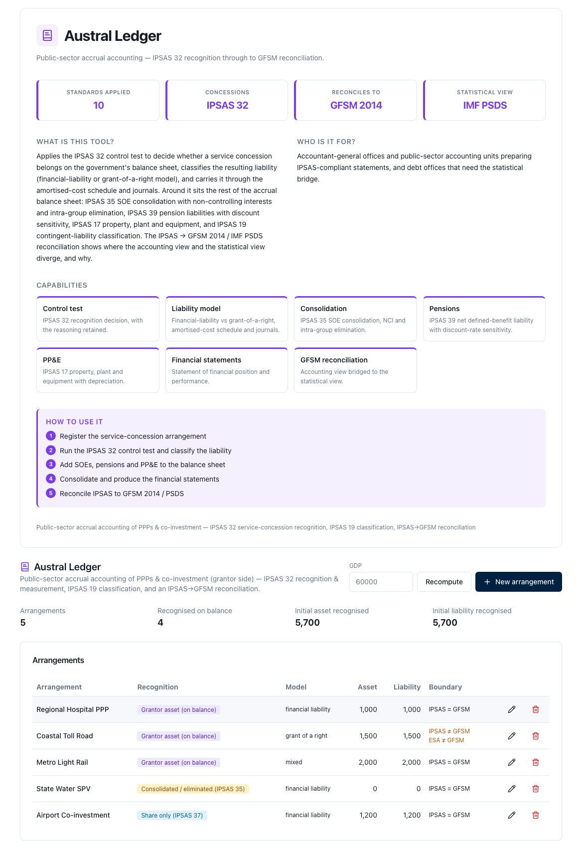
Platform module that runs the method: Austral Ledger (/ipsas) — public-sector accrual accounting on the grantor's side. Screens: portfolio home and recognition schedule (ipsas), arrangement create and edit (ipsas/arrangements/new, ipsas/arrangements/<id>), consolidated IPSAS 1 statements (ipsas/statements), IPSAS 35 public-enterprise consolidation (ipsas/consolidation, reading M6's portfolio), IPSAS 39 pensions (ipsas/pensions), IPSAS 17 PP&E (ipsas/ppe), IPSAS 45 and DBO disclosure (ipsas/ipsas45), and the on-screen manual (ipsas/manual). By API: arrangement compute (POST /ipsas/compute), valuation at a reporting date (POST /ipsas/reporting-date), and the XLSX disclosure package (GET /ipsas/reports/xlsx, lang=en|es)
Languages: English (this edition) and Spanish · HTML and PDF at austral‑intelligence.com/manuals
This manual explains how a government accountant decides, arrangement by arrangement, what a portfolio of service concessions puts on the State's books — how much, on which line, and on what schedule — and why that figure so rarely matches the one the same State publishes as debt. Its thesis is that control is the widest net: the accounting recognition test asks whether the grantor controls the public service, which is the very reason a State signs a concession, so on a faithful reading almost every concession passes it; the statistical tests that decide the published debt figure ask instead who carries the risk, and recognize far less — with the consequence that the measure a government most wants to look good on is precisely the one that captures the smallest share of what the balance sheet actually holds. It presents grantor-side concession accounting as a self-contained eleven-step method running from perimeter to governance, built on IPSAS 32 for the control test, IPSAS 19 for the contract's guarantees and IPSAS 1 for where the figures land, reconciled against the IMF's GFSM 2014 and against ESA 2010 with Eurostat's Manual on Government Deficit and Debt and the Eurostat–EPEC Guide — the third and strictest boundary, the only one of the three under which a single minimum-revenue guarantee of any size consolidates the arrangement onto the government's balance sheet by itself. It walks the eleven steps through a five-arrangement demonstration portfolio of the fictitious Republic of Lemuria — a hospital, a toll highway, a light rail line, a State-owned water utility and an airport joint venture — with every figure shown, including the toll highway's deliberate case where the three boundaries give three different answers on the same contract; a companion box reads the same method against real, cited Chilean toll-concession instruments. It shows how the method runs on the Austral platform, screen by screen, declaring where the tool still falls short of the method it implements; and it explains why this particular method — not the arithmetic of a single amortization schedule, but the discipline of closing forty concessions every year against three rulebooks that do not agree — breaks in a spreadsheet. It is written for government accountants, debt offices, statistics offices, public-private-partnership units, comptrollers and auditors.
Austral Intelligence (2026). Accounting for Service Concessions: The Grantor's Side. Manual M8, Austral Manual Series, version 1.0, September 2026. https://austral-intelligence.com/manuals/service-concession-accounting/
Every figure in the worked example (section 4) and in the screenshots (section 5) is generic: it belongs to the fictitious Republic of Lemuria's five-arrangement demonstration portfolio, shipped as a demonstration pack in the platform and calibrated so the method can be followed from start to finish. None of it comes from a client or a real project, and none of it should be used as a reference for the assets, liabilities or debt of any actual concession portfolio. GDP for the worked example is a declared assumption (60,000, in millions of Lemuria's currency), and every "% of GDP" figure in the manual carries it alongside; none of the method's decisions depend on it. The provision ceiling on discount accrual (section 2.4, section 3 Step 7) and the imputed-loan conventions used in the statistical bridge (section 2.7, section 3 Step 9) are declared as Austral calibrations and not as published rules of any cited source. The methodologies cited are credited to their authors — IPSASB, the International Monetary Fund, and Eurostat with the European PPP Expertise Centre; the only product name in the manual is Austral.
This is the first English edition of Manual M8, translated from the Spanish version 1.0 (25 September 2026). Every figure, table and citation is carried over unchanged; where the two editions differ, including after a future correction to either one, the Spanish edition is the reference. Where the Spanish edition cites the official Spanish-language IPSASB translation for a term or a paragraph, this edition cites the official English IPSASB Handbook directly; section 2's note on terminology says what that substitution carries over and section 7 flags the individual citations it could not independently re-verify against the English edition.
A government accounting office has, in addition to the budget, a portfolio of concessions. A hospital paid by availability, a toll highway, a light rail line that charges a fare and also receives a subsidy, a water utility operated by a company of the State itself, a co‑invested airport. The contracts are signed, the sector ministry administers them, the public‑private partnership unit negotiated them, and the debt office knows how much it committed to pay for them. What almost never exists is the answer to the accounting office's question: what part of that portfolio enters the State's books, for how much, on which line and with what profile over time — and why that figure does not match the one the same State publishes as debt.
The manual's thesis fits in one sentence, and it is worth stating before the method. Control is the widest net. The test that decides the accounting recognition of a concession is a test of control over the public service, and controlling the public service is the very reason a State signs a concession: on a faithful reading of the standard, almost every concession passes it. The tests that decide statistical recording are tests of risk, and they recognize less. From this follows the consequence that orders the whole manual: the measure by which the government most wants to look good — its debt figure, the one that anchors the fiscal rule — is precisely the one that recognizes less of what the balance sheet contains. This is not a suspicion: it is the arithmetic of two rule books that do not say the same thing, and one of the two admits it in writing (§2.3, with the footnote from the European manual).
The question is: what part of this concession enters my books, for how much and on which line? The product is a register of accounting recognition and measurement on the grantor's side: each arrangement with its reasoned recognition decision, its initial asset and liability, the development of the liability year by year, the depreciation of the asset, the classification of its guarantees, the position at the reporting date and the bridge to the statistical figure.
From this follows, just as clearly, what it does not answer.
What this register is not
- It is not a project appraisal. It does not say whether the concession was worth doing, whether value for money was positive, or whether the payment mechanism is well designed. A poorly appraised contract is accounted for just as well as a well‑appraised one, and that is precisely why accounting does not substitute for appraisal (M1).
- It is not the commitments register. How much the State committed to pay under the contract — the annual profile and its present value — is a contractual flow, and it is a different manual (M2). This one measures a recognized stock at amortized cost, which is a different figure from the same contract. The full boundary is set out in 1.2.
- It is not the valuation of the guarantee. Pricing the probability that a minimum revenue guarantee will be called requires a loss distribution, and that is M7. This manual consumes that price, classifies it — a recognized provision or a disclosed contingent liability — and develops it through to closing. It does not re‑derive the distribution, and it says so every time it publishes the figure.
- It is not the fiscal risk statement. Consolidating every family of risk, correlating them and setting a ceiling on them is M9. This manual hands it two families — provisions and disclosures — and deliberately does not hand it the recognized direct liability, because that line already belongs to the commitments register, and reporting it here would count it twice.
- It is not the operator's accounting. The standard that governs this manual says nothing about the other side of the contract: the operator is accounted for under the mirror private‑sector standard (§2.1). The two sides of the same contract are written in two different books, and confusing them produces the error of believing that what the operator capitalizes is what the State recognizes.
- It is not the rest of the public sector's balance sheet. The consolidation of public enterprises, pensions, property and infrastructure are other standards in the same suite and other manuals (M6 and its own). They enter here only as the place where the concession's figures land (§2.5) and as the boundary that Step 0 has to draw.
There is an asymmetry worth flagging in advance because it orders the whole method: of the decisions the manual makes about a contract, three are boundaries and one is a classification, and they are confused all the time. The three boundaries — control, economic ownership, risks and rewards — decide whether the asset and the liability enter, each into a different book. The classification of the financial liability model decides what kind of liability it is, and it depends on a single thing: who pays. A contract can be fully on the State's accounting balance sheet with a liability that is not debt under any statistical standard, and that is not an anomaly: it is the most common case in Latin America, the toll concession.
This is the most costly confusion in this discipline, and it deserves its own section because both figures exist, both are correct, and they are not the same.
The commitments register asks what did I promise. It takes the contract, reads the payment mechanism, and publishes the annual disbursement profile and its present value; alongside it, what the State could owe if a guarantee is called. It is a register of contractual obligations, and its natural unit is the flow.
The grantor's accounting asks what do I have and what do I owe. It takes the same contract, decides whether the infrastructure asset belongs to the State, recognizes it at fair value, recognizes a liability of the same amount against it, and then develops it: each payment is split into finance charge, principal amortization and service expense, until the liability is extinguished. Its natural unit is the stock at amortized cost, which starts at the asset's fair value and ends at zero.
The two measure the same contract and never coincide. On the hospital from the §4 example — an asset of 1,000, twenty‑five payments of 95 of which 15 is service — the whole‑life commitment is 2,375 in nominal flow; the recognized liability at inception is 1,000; the finance charge over the whole life is 1,000 and the service expense is 375. The three figures describe the same contract and none is the sum of the others. And there is a fourth: what that contract puts into statistical debt, which is the far shore of Step 9, and which can be 1,000, can be zero, and can be an amount that accounting does not measure anywhere.
The no‑duplication rule that follows from this is a matter of nature, not of inventory: the consolidated register takes the commitment from one manual and the recognized liability from the other, and never the two as if they were two obligations. Whoever tries to add them together gets a figure that means nothing and that, invariably, someone cites.
The common formulation of this manual's tension — "the accounting standard recognizes and the statistical one does not always" — points in the right direction and falls short. What needs to be said precisely is why it recognizes more, and the reason lies in each test's trigger.
The accounting test asks whether the grantor controls or regulates what services the operator provides with the asset, to whom and at what price, and whether it controls any significant residual interest at the end. Both conditions are met in the normal design of a concession: the State sets the maximum tariff and its adjustment formula because that is the reason it tenders a public service, and the works revert to the State because that is the reason it is a concession and not a sale. Who financed the works is irrelevant to this test, and the standard itself says so.
The statistical tests ask something else: who bears the risk. The asset leaves the State's balance sheet when the private partner bears the construction risk and, in addition, either the availability or the demand risk — with the caveat that a nominal transfer of availability risk does not count if the deduction mechanism does not put the operator's revenue at stake. And it returns to the balance sheet under any of the secondary reconsolidation provisions: majority public financing of capital expenditure, State guarantees on most of the debt, termination compensation that repays creditors, residual value transferred below market. The European version adds a rule the International Monetary Fund's version does not have: any minimum revenue or minimum demand guarantee consolidates on its own.
Those two questions cannot give the same answer, and the §4 example teaches it with a figure. The toll highway in the example — the operator builds, bears the demand risk and lives off the toll, backed by a minimum revenue guarantee — gives three results on the same contract: under the control test it is an asset of the State, with 1,500 of asset and 1,500 of unearned revenue on its books; under the International Monetary Fund's economic ownership test it stays with the operator, and its contribution to statistical debt is zero; under the European test it returns to the State's balance sheet under the guarantee rule, with an imputed loan of 1,500 of gross debt. The same concession, the same day: 1,500 of accounting liability that is not debt, zero debt under one statistical book and 1,500 of debt under the other. The difference between the two statistical shores of the same contract is 1,500, and it is not an error: it is the subject of Step 9.
This is the reading Austral's own work supports. The Recognition Rule measures the distance between what the rule binding a jurisdiction obliges it to recognize and the economic tail the sovereign actually carries, and it does so with four separate lenses on the same contract; this manual runs three of them — the three boundaries of Step 2 — and refers the fourth, the economic one, to M2 and M7. The Useful Silence explains why the liability tends to go unvalued, and who benefits from that. The Anchor and the Perimeter shows what happens when the fiscal anchor is tied to the measure that recognizes less. And The Third‑Party Guarantee Decision is the boundary of Step 7: the guarantee is valued on the distribution and not on the average path, and here that price is consumed, not recalculated.
It is not a decision instrument: it is a closing instrument. It runs at three moments, and all three are calendar‑ or event‑driven, never tender‑driven.
At the start of each arrangement, once, when the grantor obtains control of the asset: perimeter, control test, the two statistical boundaries, initial measurement, liability model and the first schedule. It is the only moment in the method that resembles a project.
At each year‑end close, for the whole portfolio: the period's finance charge and amortization, the depreciation, the review of each provision and each disclosure, both sides of the statement at the same date, the notes and the bridge to the statistical figure. Together with the commitments register (M2) and the public enterprise diagnostic (M6), it is one of the three manuals in the series that run every year and not once per transaction.
Before every event, outside the calendar: a contract modification that remeasures the asset and the liability, an indexation, an impairment, a guarantee call, an early termination, a handover to the State. Step 10 exists for that, and its rule is that an event does not wait for closing: it opens a dated version of the register.
The annual product feeds three calendars that are not its own: the reporting entity's financial statements, which are its natural destination; the debt office and the statistics office, through the bridge of Step 9; and the fiscal risk statement (M9), to which it hands its provisions and its disclosures, and not its direct liability.
Six readers and six uses of the same register. It is worth listing them because none reads the same column, and the register has to serve all of them.
Two caveats about this division of labor. The first: the boundaries of Step 2 are not decided by whoever operates the tool. Deciding that a contract is the State's economic ownership has consequences for the country's published debt; the analyst applies the test, documents the result and takes it to whoever is responsible for setting it formally. The second: recognition is not a matter of opinion, but it is a matter for discussion. A control test resolved with "yes" and no written basis is not an accounting decision, it is a preference; the method requires the reason, and §3 requires it at every step.
For each arrangement and for the portfolio, the method produces five figures and a list. The six go together: published separately, any of the first five is misread.
Three of these figures — the recognized liability, the contractual commitment and statistical debt — measure different things about the same contract, and the manual never adds them together or presents them as the same thing. It is the rule §3 repeats at five different steps because it is the one most often broken.
Three things, in the order of the series.
A self‑contained method. §3 develops eleven steps — from the perimeter to governance — with what goes in, what comes out and what the decision rule is at each one, and closes with the reviewer's checklist. It is written to be run with any tool: a spreadsheet, a folder of evidence and the contract are enough, and that is the condition that later lets §6 show where that spreadsheet breaks. §2 credits each rule to its source with paragraph — the concession standard on the grantor's side, the provisions standard, the presentation standard, the International Monetary Fund's government finance statistics manual with its debt guide, and the European system of accounts with its deficit and debt manual and the joint guide with the European centre of expertise — and states where the sources do not agree and what position the manual takes.
A reproducible example. §4 walks the eleven steps through a portfolio of five arrangements that is a deliberate sample: the five possible recognition outcomes, one per arrangement, and one of them — the toll highway — with the three boundaries giving three different answers, which is the manual's thesis in figures. Never client data. A separate box carries the Chilean counterpoint with primary sources from the concessions corpus.
The tool that runs it, and that the client keeps. §5 shows the module screen by screen, with what it records, what it exports and what it still does not do, stated as such and not omitted. §6 is honest about the spreadsheet argument: a spreadsheet develops a liability at amortized cost perfectly well — it is a textbook exercise — and what the manual discusses is not that calculation, but what happens to a spreadsheet when it stops being a calculation and becomes the book of forty concessions that has to be closed every year, reconciled against two further rule books and handed to whoever audits it. §7 gathers the references with their verification status.
Anyone who only needs to know whether a concessions register that has come to them for sign‑off is done correctly can go straight to the reviewer's checklist at the close of §3. Anyone who wants the logic in one page, to summary 3.11.
Every rule of the method in §3 comes from an accounting standard binding on whoever prepares the statements, from a statistical rule book that decides what debt figure the country publishes, or from a national practice that has tested both. This section says where each one comes from, with paragraph, so the reviewer can argue the rule at its source and not in the manual. The split is four bodies. One accounting rule book: IPSAS 32, Service Concession Arrangements: Grantor, with IPSAS 19 for the contract's guarantees and contingencies and IPSAS 1 for where the figures land. Two statistical rule books: the International Monetary Fund's Government Finance Statistics Manual 2014 (GFSM 2014), with its public-sector debt statistics guide; and ESA 2010 with Eurostat's Manual on Government Deficit and Debt (MGDD) and the 2016 Eurostat–EPEC Guide on the statistical treatment of public-private partnerships. And the private-sector mirror, IFRIC 12, which matters because it is the one with a decade of published evidence and because IPSAS 32 itself states it was written to mirror it. Table 2.8 links each step of §3 to its source and to the §5 screen that runs it.
A reading warning, at three points where the sources do not agree, and the manual takes a declared position, not an invented consensus.
(i) Whether the accounting test and the statistical test reach the same answer. GFSM 2014 states that its approach "is broadly consistent with considerations listed by the International Public Sector Accounting Standards Board (IPSASB) for the recognition and measurement of a service concession asset" and that the considerations of one and the other "should, in principle, lead to the same conclusions on economic ownership" (¶A4.63, with footnote 16 naming IPSAS 32). Eurostat holds the opposite, and writes it in a footnote of its own manual: "if IPSAS rules were applied, almost all existing PPPs in the Member States would end up in the balance sheet of government because the main criteria to be taken into account for their classification would be the control of the assets and the allocation of the assets at the end of the period of the contract. However, ESA 2010 stresses the concept of economic ownership and not the one of legal ownership" (MGDD 2019, §6.4.1 ¶4, footnote 214; MGDD 2022, same section, footnote 284). The two rule books do not say the same thing about each other, and the manual takes Eurostat's position because it is the one the arithmetic confirms: the control test recognizes more, and section 2.1 explains why it has to be that way.
(ii) Exactly where the line of public financing sits. The MGDD writes it as majority: "if the majority of the financing of the capital expenditure would be provided by government […] the asset must be classified on its balance sheet" (¶55). The Eurostat–EPEC Guide writes it as an arithmetic threshold: "if a government commitment of financing or any other support amounts to 50% or more of the capital expenditure to be incurred for the construction of the asset, the PPP is automatically recorded ON BALANCE SHEET for government" (theme 14.4). A contract financed exactly fifty-fifty falls on one side under one wording and the other under the other. The manual publishes the Guide's threshold — 50% or more — and says so, because it is the operative formulation and the stricter of the two.
(iii) Which rate develops the liability. IPSAS 32 sets a hierarchy: the finance charge "is determined based on the operator's cost of capital specific to the service concession asset, if this is practicable to determine" (¶AG40), and only if that is not practicable is "the rate implicit in the arrangement […], the grantor's incremental borrowing rate, or another rate appropriate to the terms and conditions of the arrangement" used (¶AG41). Practice — and the §5 tool — starts from the implicit rate, which the standard places second. It is an inversion of the hierarchy, declared here, repeated in Step 5 and in §5, and it has its reason: the operator's cost of capital is rarely observable to the grantor, while the payment schedule always is. But the reason does not erase the standard's order, and a preparer who can determine the operator's cost of capital must use it.
And a warning on method. This manual credits methodologies that are not its own and does not use them as a product name: IPSASB for IPSAS 1, 19, 32, 35 and 37; the International Monetary Fund for GFSM 2014 and the public-sector debt guide; Eurostat for ESA 2010, the MGDD and the joint guide with EPEC. The only product name in this manual is Austral. Where the method described here departs from its source, it says where and why; where a quote could not be verified against the document, it is marked [to be verified] in §7 and not asserted in the body.
A word on terminology. This manual quotes the official IPSASB Handbook of International Public Sector Accounting Pronouncements directly, in English, with paragraph citations — ¶AG for the Application Guidance appendix, as numbered in the Handbook. From that Handbook come the terms used throughout: service concession arrangement, service concession asset, operator, financial liability model, grant of a right to the operator model, finance charge, carrying amount, provision, contingent liability, disclosure, best estimate, expected value, non-controlling interest and accrual basis of accounting. The official Spanish edition this manual's Spanish original follows denotes these same standards as "NICSP" rather than "IPSAS" — NICSP 32 is IPSAS 32 — a labelling difference with no bearing on the English text below. Three terms in this section have no single fixed form in the Handbook's own prose and are used here for economy of language, alongside the standard's own wording the first time they appear: control test (¶9 states two conditions rather than naming a test); unearned revenue (the standard's own phrase is "the unaccrued portion of the revenue"); and division of the arrangement [to be verified] (used here as a plain description of the mechanism in ¶27–28, since this manual could not independently confirm the Handbook's own official heading for that paragraph range).
The standard applies to the entity that "prepares and presents financial statements under the accrual basis of accounting" (¶2): it is an accrual-basis standard, and a State that runs on cash has nothing to recognize here — it does, however, have everything to disclose. Outside its scope are arrangements "that do not involve the delivery of public services" and those with service and management components "where the asset is not controlled by the grantor (e.g., outsourcing, service contracts, or privatization)" (¶6). And the standard says nothing about the operator's accounting (¶7): that is IFRIC 12's, which is why the two sides of the same contract are written in two different books.
The two conditions. The grantor recognizes as a service concession asset what the operator contributes — and any improvement to an existing asset of the grantor's — if, and only if, both are met:
"(a) The grantor controls or regulates what services the operator must provide with the asset, to whom it must provide them, and at what price; and (b) The grantor controls—through ownership, beneficial entitlement or otherwise—any significant residual interest in the asset at the end of the term of the arrangement." (¶9)
And the proviso that in practice resolves half the cases: when the asset is used within the arrangement for its whole useful life — a whole-of-life asset —, condition (a) alone is enough; the standard applies "if the conditions in paragraph 9(a) are met" (¶10). It is not that the residual condition is deemed met: it is that for that asset the standard does not require it, because at the end of the arrangement there is no residual interest left to control.
What is control and what is not, in the application guidance, which is where the standard is actually decided:
Initial measurement. The asset is measured initially at fair value (¶11); when what enters the arrangement is an existing asset of the grantor's that meets the conditions, there is no new recognition but reclassification (¶12), and once recognized or reclassified the asset is accounted for under IPSAS 31 or IPSAS 45 as appropriate (¶13). Practical consequence Step 3 records: the asset is not recognized at the operator's cost or at the contract's value, and reclassifying an asset the grantor already owns does not create a liability (¶14), except for any additional consideration the operator contributes (¶15).
Why this test recognizes so much. Because its trigger is control of the public service, and controlling the public service is the very reason a State signs a concession. A contract in which the State did not specify what service is provided, to whom and at what price would not be a service concession arrangement: it would be something else. Hence, on a faithful reading of ¶9, ¶10 and ¶AG7, almost every concession passes the control test — and this is not this house's own reading: it is exactly what Eurostat writes in the footnote quoted above when it says that under IPSAS rules almost all existing public-private partnerships in the Member States would end up on government's balance sheet. The statistical tests, by contrast, are tests of risk, and risk does transfer. That structural difference — control versus risk — is the subject of the whole manual, and section 2.3 writes it out with its paragraphs.
Once the asset is recognized, the grantor also recognizes a liability (¶14), measured initially at the same amount as the asset, adjusted for any other consideration between the parties (¶15). Up to there, there is no choice. The choice comes after, and it is a second classification, independent of the first:
"The nature of the liability recognized is based on the nature of the consideration exchanged between the grantor and the operator." (¶16)
The grantor may compensate the operator "by any combination of: (a) Making payments to the operator (the 'financial liability' model); (b) Compensating the operator by other means (the 'grant of a right to the operator' model)" — the right to charge third-party users, or access to another revenue-generating asset, "e.g., a private wing of a hospital […] or a private parking facility adjacent to a public facility" — (¶17). The model is decided by who pays, not by who bears the risk. It is the distinction this manual repeats most often, because confusing it with the control test is the most common error in a concessions register: the same contract can be on balance sheet under IPSAS 32 and carry a liability that is not debt under the statistics, and that combination — perfectly correct — produces half of Step 9's bridge.
The financial liability model (¶18–23, ¶AG37–AG46). It applies "where the grantor has an unconditional obligation to pay cash or another financial asset to the operator for the construction, development, acquisition, or upgrade of a service concession asset" (¶18). The obligation is unconditional when the grantor has guaranteed to pay the operator:
"(a) Specified or determinable amounts; or (b) The shortfall, if any, between amounts received by the operator from users of the public service and any specified or determinable amounts referred to in paragraph 19(a), even if the payment is contingent on the operator ensuring that the service concession asset meets specified quality or efficiency requirements." (¶19)
Two large consequences follow. The first: a performance deduction does not remove unconditionality. An availability payment subject to deductions for failure is still a financial liability, because the conditionality falls on the quality of the service and not on the existence of the payment. The second, and it is the one that crosses this manual with M7: a minimum revenue guarantee turns a user-pays contract into a financial liability for the guaranteed amount, under ¶19(b), and it does so in the accounts of any jurisdiction applying IPSAS 32 — not only in Europe. The standard adds that the obligation is unconditional when the grantor "has little, if any, discretion to avoid the obligation usually because of the binding arrangement with the operator being enforceable by law" (¶AG37).
Splitting each payment is Step 5's operative rule: payments to the operator are allocated "according to their substance as a reduction in the liability […], a finance charge, and charges for services provided by the operator" (¶21), and the finance charge and the charge for services are expense (¶22). The liability recognized "does not include the finance charge and service components of the payments" (¶AG38). When the asset and service components are separable, the service is allocated by relative fair values; when they are not, by estimation techniques (¶23). The service component "is ordinarily recognized evenly over the term […] because this pattern of recognition best corresponds to the service provision" (¶AG46). And once the rate is fixed, it "may not be subsequently changed unless the asset component or the whole of the arrangement is renegotiated" (¶AG44) — which is why a contract modification requires remeasurement and not a silent adjustment of the schedule (Step 10).
The grant of a right to the operator model (¶24–26, ¶AG47–AG49). It applies when the grantor has no unconditional obligation to pay and grants the operator the right to charge third-party users or access to another revenue-generating asset: the liability is then accounted for "as the unearned portion of the revenue arising from the exchange of assets between the grantor and the operator" (¶24). This manual shortens that to unearned revenue — a house term, declared above — and it is the word that carries the most weight in it, because it is the liability the reader does not recognize as a liability. The exchange "is regarded as a transaction that generates revenue," but because the right granted runs for the term of the arrangement, the grantor does not recognize the revenue immediately: it recognizes a liability for the portion not yet earned and reduces it as the revenue is earned (¶26).
By what pattern is it released? The standard says "according to the economic substance of the service concession arrangement" (¶25), and the guidance states what the normal substance is: "usually as access to the service concession asset is provided to the operator over the term of the service concession arrangement" (¶AG47). Straight-line release over the term is, then, the standard application of the rule and not a simplification the tool makes — with an exception ¶AG47 writes expressly: when the operator combines third-party charges with grantor payments and third-party revenue significantly reduces or eliminates those payments, "another basis may be more appropriate for reducing the liability." A register using the straight-line basis must verify that this exception does not apply, and say so.
¶AG49 closes a door that is often confused: shadow tolls. When the grantor pays the operator solely for third-party use of the asset, that payment "is compensation in exchange for the usage and not the acquisition of the service concession asset"; it does not reduce the ¶24 liability and is accounted for as expense. A shadow toll that also pays for construction is something else, and the two have to be separated.
Division of the arrangement — mixed consideration (¶27–28, ¶AG50). The standard's own heading for this case is division of the arrangement; "mixed consideration" is this house's shorthand for the economic fact that produces it — two forms of consideration in the same contract. When the grantor pays for the works "partly by incurring a financial liability and partly by the grant of a right to the operator, it is necessary to account separately for each part of the total liability" (¶27), and each part is accounted for under ¶18–26 (¶28). The initial amount of the total liability is still the one in ¶15 — the same as the asset's —; what is split is its nature, "each portion of the liability […] recognized initially at the fair value of the consideration paid or payable" (¶AG50). This is the case of the hospital paid both by availability and by activity, and of the light rail line in the §4 example.
Other liabilities and other revenue. The grantor accounts for the arrangement's other liabilities, commitments, contingent liabilities and contingent assets under IPSAS 19, IPSAS 28, IPSAS 30 and IPSAS 41 (¶29) — the detail is section 2.4 — and revenue other than that of ¶24 under the applicable standards (¶30). ¶29 is also the paragraph that separates the concession's recognized liability — the one born in ¶14–15 — from the same contract's contingent liability: the first is an on-balance-sheet liability and does not enter the contingency note; the second goes under IPSAS 19. The guidance splits the guarantees: those meeting the definition of a financial guarantee contract go under IPSAS 28, 30 and 41 (¶AG52); those that do not and are not insurance contracts go under IPSAS 19 (¶AG53); and contingencies arising from disputes over the terms of the arrangement, also under IPSAS 19 (¶AG54). In the opposite direction, IPSAS 41 ¶2(k) excludes from its scope the rights and obligations of an IPSAS 32 arrangement, except for the derecognition of the financial liability the grantor recognizes under the financial liability model, which is governed by IPSAS 41. Where it is the operator that pays the grantor for access to the asset, the standard addresses that too: upfront payment, a payment stream or other consideration (¶AG55–AG60).
This is the manual's most consequential section, because its result is not a rating: it is what debt figure the country publishes. Accounting decides what enters the financial statements; statistics decides what enters the gross debt that anchors the fiscal rule. They are two different questions, with two different tests, and there are two statistical rule books, not one.
A public-private partnership is, for the GFSM, a long-term contract under which one unit acquires or builds an asset, operates it for a period and hands it over to a second unit (¶A4.58). The decision on which balance sheet it is recorded on "is not straightforward," and the manual explains why: the contract usually allows government to specify design, quality, capacity use and maintenance, and "typically, the assets have service lives much longer than the contract period so that, for this reason alone, the government will control the assets, bear the risks, and receive the rewards for a major portion of the assets' service lives" (¶A4.61). The GFSM thus recognizes the very same fact that drives the control test.
But its test is a different one: "the statistical treatment depends on the economic ownership of the asset(s) involved. In macroeconomic statistics, a distinction is made between legal ownership and economic ownership […] based on risks and benefits" (¶A4.62). Box A4.4 lists the factors to consider, in two families — those associated with acquiring the asset (the degree to which government controls design, quality, size and maintenance; construction risk) and those associated with using it (supply risk, demand risk, residual value and obsolescence risk, availability risk) — with the caveat that "it is not possible to state prescriptive rules that will be applicable to every situation" and that "majority" must be assessed economically: "a single risk and reward may imply the 'majority' in some cases, while in other cases, a number of separate risks and rewards combined may do so" (footnote 15).
The treatment when government is the economic owner is ¶A4.64, and it is what makes Step 9's bridge more than a subtraction: if government is the economic owner throughout the contract and pays nothing at inception, "a transaction must be imputed to cover the acquisition of the asset(s). […] Most frequently, these contracts will be recorded as the acquisition of the asset through an imputed financial lease because of the similarity with actual financial leases," or else a loan equal to the asset's market value is imputed at acquisition and government's payments are split between loan amortization and expense. If the private corporation is the economic owner, the debt associated with the acquisition is attributed to it (¶A4.65).
And the point where the GFSM speaks of IPSAS. ¶A4.63 holds that "the macroeconomic statistics approach is broadly consistent with considerations listed by the International Public Sector Accounting Standards Board (IPSASB) for the recognition and measurement of a service concession asset," that IPSAS's considerations on control "include aspects of risks and rewards, and should, in principle, lead to the same conclusions on economic ownership." This manual's method does not endorse that statement, and it says so with the argument, not the opinion: IPSAS 32's test is satisfied by regulation of the service and of the price (¶9(a), ¶AG7) with no regard to who financed it (¶AG3(d)), while the statistical test looks precisely at financing, guarantees and the term. Two tests that ignore different variables cannot converge except by coincidence. The GFSM's own box A4.5 hints at this when it describes European practice as one operationalization among others.
What is debt and what is not. Total gross debt "consists of all liabilities that are debt instruments. A debt instrument is defined as a financial claim that requires payment(s) of interest and/or principal by the debtor to the creditor at a date, or dates, in the future" (¶7.236), and the list is closed: special drawing rights; currency and deposits; debt securities; loans; insurance, pension and standardized guarantee schemes; and other accounts payable. Everything on the GFS balance sheet is debt except equity and financial derivatives with share-purchase options (¶7.237). Hence the consequence Step 9's bridge turns into a single line: unearned revenue under the grant of a right model is not statistical debt — it is not a financial claim requiring the payment of interest or principal, but unearned revenue. A register that adds a toll concession's accounting liability to gross debt is adding together two things the very definition keeps apart.
The European version of the risk test is the strictest of the three boundaries, and it is the only one that also publishes a closed list of clauses that bring the asset back onto the State's balance sheet.
The primary gate. The assets of a public-private partnership are classified on the partner's balance sheet and not on government's if three conditions are met: that the partner bears construction risk; that it bears at least one of availability or demand risk; and that the risks "are not incurred by government through other means, such as through (e.g.) government financing, government guarantees and early redemption clauses" (MGDD 2019, §6.4.1 ¶5–6). The rule calls for a majority of risks and rewards, not all of them (§6.4.3.2 ¶35–36, citing ESA 2010 ¶20.283), and it admits that government may bear exceptional risks — force majeure, archaeology, land registry, environment, public safety — without that moving the classification.
The weak-deductions proviso, which is the one that stops the transfer of availability risk from being nominal: penalties must be "automatic (i.e. clearly stated in the contract and not subject to bargaining or to a decision by government on whether to apply them or not)," must have a significant effect on the partner's revenue or profit and not be merely symbolic, and in the event of non-negligible unavailability government's payments must fall to zero, "according to a fundamental principle 'zero availability — zero payment'" (§6.4.3.2 ¶49). A contract with a weak deduction regime does not transfer availability, whatever it says.
The secondary reconsolidation provisions, which operate "independently from the analysis of the risks mentioned above" (§6.4.3.2 ¶51):
And the rule the method must run, and that almost no register runs: the tests are done together. "For the evaluation of the risk distribution between government and the partner, both tests for majority financing and guarantees in relation to the capital expenditure of the PPP project must be undertaken jointly. It might well be the case […] that government would provide a minority of the total capital expenditure, but would then guarantee a major part of the remaining project finance […]. In this case, if the combined effect of government support would represent more than a majority of capital expenditure, this would lead to the conclusion that a majority of risks would be incurred with government" (§6.4.3.4 ¶69). It is the same additivity principle the manual states at the start of the chapter: the criteria "should not be considered in isolation, criteria by criteria, but according to a principle of additivity" (§6.4.2.3 ¶27–28). A contract with 40% public financing and 40% guaranteed debt passes each provision separately and fails the joint test. Step 2 asks for this explicitly, and §5 declares where the tool today still reads provision by provision.
Concessions, which is the Chilean case. The MGDD treats separately contracts in which government makes no regular payments, or these are not the majority of the partner's revenue: there the asset may be recorded on the corporation's balance sheet (2019, §6.3.1.5.2 ¶23). But if government finances the majority of the construction cost, or guarantees more than 50% of the debt allocated to the asset, the asset returns to the State's balance sheet (¶24). And above all:
"If in the initial contract or in the course of its lifetime, government provides a minimum revenue guarantee (such as on a minimum volume of traffic) or, in some cases, a minimum level of profitability of the concessionaire (for instance in terms of return on equity), government should be considered to bear the majority of the economic risks and the assets should be recorded on government balance sheet. Under this perspective, the main distinction between concessions and PPPs falls." (MGDD 2019, §6.3.1.5.2 ¶25)
The 2022 edition of the same manual keeps the rule, renumbers it as §6.3.1.5.2 ¶43 and hardens it: the assets must be recorded on government's balance sheet "without exception." It is the only one of this section's quotes whose text changed between editions, and it changed to become stricter.
The 2016 Eurostat–EPEC Guide takes that rule to its most categorical form, and it is the sentence that governs Step 2:
"Eurostat's view is that any form of minimum use or minimum revenue guarantee does influence the statistical treatment and automatically leads to the PPP being ON BALANCE SHEET for government." (theme 4.10.3)
Theme 14.5 repeats the rule for State support outside the payment mechanism — minimum-use or minimum-revenue guarantees, "whether as a specific undertaking or in the payment mechanism" — and adds the useful exception: a guarantee limited to the authority's own compliance with its contractual obligations does not affect the statistical treatment. Theme 4.9 closes the tariff-tiering escape route: a unit price in the low usage band that is in fact equivalent to a minimum-use or minimum-revenue guarantee brings the contract onto the balance sheet all the same.
And the accounting consequence of crossing the boundary, which is Step 9's second bridge. When the asset is recorded on government's balance sheet, the capital expenditure is gross fixed capital formation and "the financial account would match the capital expenditure by an imputed government liability, which would increase government gross debt when recorded as an imputed loan (AF.4)" (§6.4.2.3 ¶24). That imputed loan "at inception is equal to the gross fixed capital formation" (§8.2.2.2), its principal "must be spread over the entire period with no impact on government net lending/borrowing (B.9), while imputed interest must also be calculated and included in government expenditure" (§6.4.2.3 ¶26), and its service is split into a financial flow repaying the principal (F.4) and a non-financial flow of interest (D.41), by analogy with a financial lease (§6.3.1.4 ¶12). In a concession with a minimum revenue guarantee the chain closes fully: ¶25 requires treating the contract "similarly to a procurement for the construction of the assets," and §6.4.2.3 ¶24 says what that purchase produces in the accounts — government's gross fixed capital formation and an imputed loan that increases its gross debt. The same figure — "an imputed debt as a counterpart" — appears in the manual's footnote 211, though for a different case: that of the public concessionaire that lacks decision-making autonomy and whose concession assets are reclassified onto the balance sheet of the contracting or controlling government unit. The two should not be confused: the imputed counterpart is the same, the trigger is not. This is the only debt figure this manual produces with no financial liability in the grantor's books, and its measurement, its assumptions and its attribution are in 2.7.
| Boundary | Source | Test | What it decides |
|---|---|---|---|
| Accounting | IPSAS 32 ¶9–¶10, ¶AG5–AG12 | Control of the service, of the recipient and of the price, and of the significant residual interest | The grantor's statement of financial position and its result |
| Statistical (IMF) | GFSM 2014 ¶A4.61–A4.65, box A4.4 | Economic ownership: who bears the majority of the risks and collects the majority of the rewards | Public-sector debt in government finance statistics |
| Statistical (EU) | ESA 2010 ¶20.283; MGDD §6.4.1 ¶5–6 and §6.4.3.3–6.4.3.7; Eurostat–EPEC Guide themes 4.10.3, 12.1, 13.2, 14.4–14.5 | Risks and rewards with a primary gate and secondary reconsolidation provisions | General government debt and deficit that anchor the fiscal rule |
All three are run on the same contract and all three are published. When they do not coincide, the difference is not an error to correct: it is Step 9's figure and the manual's thesis.
The contract's guarantees and contingencies enter through IPSAS 32 ¶29 and split into three destinations that should not be confused. Service concession arrangements "may include various forms of financial guarantees (e.g., a guarantee, security, or indemnity related to the debt incurred by the operator […]), or performance guarantees (e.g., guarantee of minimum revenue streams, including compensation for short‑falls)" (¶AG51). Those meeting the definition of a financial guarantee contract are accounted for under IPSAS 28, IPSAS 30 and IPSAS 41 (¶AG52); all other guarantees and commitments, under IPSAS 19 (¶AG53); and contingent assets and liabilities arising from disputes over the terms of the arrangement, also under IPSAS 19 (¶AG54). The method in §3 classifies under IPSAS 19 and declares that boundary: a register that treats a guarantee of the operator's debt as a disclosed contingency without having verified whether it meets the definition of a financial guarantee contract is applying the wrong standard, and this must be said before §5 shows the screen.
The recognition line. A provision is recognized when, and only when, three conditions are met:
"(a) An entity has a present obligation (legal or constructive) as a result of a past event; (b) It is probable that an outflow of resources embodying economic benefits or service potential will be required to settle the obligation; and (c) A reliable estimate can be made of the amount of the obligation. If these conditions are not met, no provision shall be recognized." (¶22)
Probable has a definition, and it is the one that sets the method's operative threshold: "an outflow of resources or other event is regarded as probable if the event is more likely than not to occur, that is, the probability that the event will occur is greater than the probability that it will not" (¶31). The same phrase governs doubt about whether a present obligation exists (¶23). And the second condition is not decorative: "except in extremely rare cases, an entity will be able to determine a range of possible outcomes, and can therefore make an estimate […] sufficiently reliable" (¶33); in the rare case where it cannot, "a liability exists that cannot be recognized" and it is disclosed as a contingency (¶34). The manual always writes the two conditions together — probability greater than half and reliable measurement — because a register that looks only at probability recognizes provisions it cannot measure.
On the other side of the line: "an entity shall not recognize a contingent liability" (¶35), and it is disclosed under ¶100 "unless the possibility of an outflow […] is remote" (¶36). The disclosure carries a brief description of the nature and, where practicable, "(a) An estimate of its financial effect, measured under paragraphs 44–62; (b) An indication of the uncertainties […]; and (c) The possibility of any reimbursement" (¶100). And the line is not a final verdict: contingencies "are assessed continually to determine whether an outflow […] has become probable," and when it has, a provision is recognized in the period in which the change occurs (¶38). That is Step 10's year-end close. The standard does not ask for disclosure at the maximum: the maximum at nominal value is the statistical rule book's convention.
Measurement. The amount recognized "shall be the best estimate of the expenditure required to settle the present obligation at the reporting date" (¶44), understood as what the entity would rationally pay to settle or transfer the obligation at that date (¶45). The technique depends on the shape of the uncertainty:
Discounting and its accrual. "Where the effect of the time value of money is material, the amount of a provision shall be the present value of the expenditures expected to be required to settle the obligation" (¶53), and "when a provision is discounted over a number of years, the present value of the provision will increase each year as the provision comes closer to the expected time of settlement" (¶54). That increase is disclosed separately: ¶97(e) requires reporting "the increase during the period in the discounted amount arising from the passage of time and the effect of any change in the discount rate" (¶55 and ¶97(e)). The rate "shall be a pre-tax rate (or rates) that reflect(s) current market assessments of the time value of money and the risks specific to the liability" and "shall not reflect risks for which future cash flow estimates have been adjusted" (¶56) — the prohibition on double counting Step 7 inherits: if the expected cost coming from the risk tool is already risk-adjusted, the rate does not adjust for it again.
The ceiling on the discount accrual, and its honest origin. The standard has no paragraph stating "the accrual of the discount can never exceed the undiscounted best estimate." The ceiling is derived from three: ¶44 measures the provision at the best estimate of the expenditure required; ¶53 discounts it when the effect of time is material, so that the present value is by construction less than or equal to that estimate; and ¶51 prohibits deliberate overstatement. Accruing the discount above the undiscounted amount produces, after enough years, a provision larger than the outflow that gives rise to it — which contradicts all three paragraphs at once. The manual writes the ceiling as an operative rule and attributes it to Austral, not to the standard, because publishing it under the IPSAS 19 label would be a false citation. Its effect is the one §6 illustrates with the minimum revenue guarantee example: it is what stops a provision of 70.00 from reaching 975.71 in year 54. A corollary of Step 7 the rule requires stating: a provision that arrives with no undiscounted amount carries no known ceiling, and the register must flag it rather than assume the ceiling is the present value itself.
Disclosure. By class of provision: the carrying amount at the start and end, additional provisions, amounts used, unused amounts reversed and the discount accrual with the effect of any rate change (¶97); plus the nature of the obligation and the expected timing of outflows, the uncertainties about amount and timing, and any expected reimbursement (¶98). And the presentation rule this manual turns into an audit criterion: when a provision and a contingent liability arise from the same set of circumstances, the disclosures are made "in a way that shows the link between the provision and the contingent liability" (¶102). A provisioned guarantee and its disclosed gross exposure are two faces of the same contract, and they are presented linked.
The grantor "shall present information in accordance with IPSAS 1" (IPSAS 32 ¶31). This section is short because the presentation standard does not decide any figure; it decides where it lands, and a single one of its rules explains the most frequent presentation error in a concessions register.
The complete set. Statement of financial position; statement of financial performance; statement of changes in net assets/equity; statement of cash flows; a comparison of budget and actual amounts when the entity makes its approved budget publicly available; notes, with a summary of significant accounting policies; and comparative information for the prior period (¶21). Names vary between jurisdictions — "the statement of financial position may also be referred to as a balance sheet" — and the standard expressly allows it (¶22).
The two faces, and why they have to articulate. The statements report "about an entity's resources and obligations at the reporting date and the flow of resources between reporting dates" (¶23). And each component carries its own time reference: it must be shown prominently, "the reporting date or the period covered by the financial statements, whichever is appropriate to that component" (¶63(c)). Hence Step 8's rule: a statement of financial position dated at the start alongside a statement of performance for the year does not articulate, and the difference between the two is exactly the depreciation, the liability amortization and the provision accrual the second one carries. A package that publishes the two faces at different dates is publishing two different contracts.
The notes. They present the basis of preparation and the specific accounting policies; disclose what other IPSAS require that does not appear on the face of the statements; and add whatever is relevant to understanding them (¶127). They are presented systematically and each item on the face is cross-referenced to its note (¶128). Significant accounting policies are disclosed in their own summary (¶132).
What IPSAS 32 requires disclosing, by arrangement. "All aspects of a service concession arrangement shall be considered in determining the appropriate disclosures": a description of the arrangement; the significant terms that may affect the amount, timing and certainty of future cash flows — "the period of the concession, re-pricing dates, and the basis upon which re-pricing or re-negotiation is determined" —; the nature and extent of rights to use specified assets, of rights to expect the operator to provide services, of the carrying amount of concession assets at the end of the period — including reclassified assets the grantor already owned —, of rights to receive assets at the end of the arrangement, of renewal and termination options, of other rights and obligations such as major overhauls, and of obligations to provide the operator with access; and the changes that occurred during the period (¶32). It is disclosed individually for each material arrangement, or aggregated for arrangements of a similar nature — "e.g., toll collections, telecommunications or water treatment services" — (¶33), and it is a disclosure additional to that required by IPSAS 31 or IPSAS 45 by class of asset.
Five jurisdictions, chosen because they publish and because they diverge from one another on something that matters for this method. Structure and practice are cited; no client figures are used. The status column says what was verified and against what, because in this section half the value lies in knowing what has not been verified yet.
| Country | Which test operates, and where it is published | Does the asset appear? And the liability? | Is the reconciliation published? | What is verified |
|---|---|---|---|---|
| United Kingdom | Accounting: IFRIC 12 — IPSAS 32's private-sector mirror — in central government accounts since fiscal year 2009-10, consolidated in the Whole of Government Accounts. Statistical: ESA 2010, with public-sector net debt as the measure | Yes in the consolidated accounts: almost all private finance initiative activity is on the accounting balance sheet. No in the debt measure: most of it stays out | Partially: the difference between the accounting figure and the statistical figure is quantified by the statistics office and by the fiscal council, but it is not published as a contract-by-contract bridge | Primary sources read. The fiscal council's figure, verified by direct reading of the report (¶7.67, p. 237); the audit office's and the statistics office's figures, with the verification recorded in Austral's own paper |
| Chile | Accounting: indirect adoption of IPSAS by CGR Resolution No. 1, of 19‑01‑2026, mandatory from 1 January 2027 for central government, regional governments and municipalities; until then, Resolutions 16/2015 and 3/2020, which it replaces, remain in force. Statistical and fiscal: the commitment and the contingency are reported by legal mandate in the annual contingent liabilities report | The concessions' minimum revenue guarantee is reported as a contingent liability, with maximum exposure and expected value — not as a recognized liability or as debt | No bridge is published between the concession's accounting figure and the debt figure | The legal mandate and the report's structure, read. ✔ the regime and the adoption timetable, by direct reading of CGR Resolution No. 1/2026. [to be verified] the specific treatment those Rules give to concession arrangements, not covered by the available extract |
| Peru | A legal ceiling on the stock of firm and quantifiable contingent commitments, with central registration at the Ministry of Economy and Finance | [to be verified] | [to be verified] | [to be verified] the public accounting framework and the treatment of concessions in the State's financial statements |
| Colombia | A contingency fund funded on contract signature; the entity perimeter is defined more by legal form than by the statistical test | [to be verified] | [to be verified] | [to be verified] the public accounting regime in force and its treatment of concessions |
| Brazil | Its own framework of accounting standards applied to the public sector, convergent with international standards | [to be verified] | [to be verified] | [to be verified] the standard equivalent to IPSAS 32, its year in force and disclosure practice |
The United Kingdom, with figures, because it is the case where the divergence was measured. The private finance initiative programme reached more than seven hundred operating contracts with a capital value of the order of £60 billion and future unitary-charge commitments of the order of £199 billion out to the 2040s, with an annual charge of £10.3 billion in fiscal year 2016-17. The two magnitudes are different and are not added together: the first is a capital stock, the second a payment stream that includes service, maintenance and finance cost. Under the accounting standards, almost all of that is on the balance sheet; under the statistics, most of it was not in the debt measure, and the two figures are published by two official institutions of the same State. The statistics office, as of March 2018: about £6 billion of contracts on balance sheet within net debt and about £28 billion off balance sheet that were not. And the fiscal council, in its July 2017 fiscal risks report, with the same net debt figure and a different total: "The WGA report PFI capital liabilities of £39 billion, while PSND includes only £6 billion that are on balance sheet in the National Accounts" (¶7.67, p. 237). In other words, £33 billion of capital liability that consolidated accounting recognizes and the debt measure does not. A third magnitude, and it is not added to the previous ones either: the £39 billion is the recognized liability in the consolidated accounts, not the contracts' capital value — which is the roughly £60 billion of the previous paragraph — nor the stream of future charges. It is §2.7's recognition gap, which no issuer publishes contract by contract and two publish in aggregate.
(Corrected 24-09-2026. Until this edition the manual wrote here that "the fiscal council had estimated, as of March 2010, an off-balance-sheet stock of just under £35 billion, close to 2.5% of GDP," taken from Austral's own paper The Recognition Rule. The July 2017 report was read in full and does not contain that figure: neither "2.5 per cent of GDP" nor "March 2010" appears anywhere in its 312 pages, and the private finance initiative is mentioned on only one page, 237. The order of magnitude holds — £33 billion against "just under £35 billion" — but the date, the percentage of GDP and the attribution do not. The manual publishes what the report says, with its page. See reference 14.)
And the fact that makes the British case an open question and not a closed episode. In October 2024 the United Kingdom changed the measure that anchors its fiscal rule: the charter for budget responsibility in force since then defines the supplementary target as "a target to ensure debt, defined as Public Sector Net Financial Liabilities (PSNFL), is falling as a share of the economy by 2029‑30" (Charter for Budget Responsibility: Autumn 2024, ¶3.7). The measure is wider than the previous one — it brings in financial assets and liabilities the net debt measure did not capture. But widening the measure does not move the recognition line, and it is worth saying precisely why: a public-private partnership the statistical test leaves off government's balance sheet generates no liability at all in national accounts, because the imputed loan of the MGDD's §6.4.2.3 ¶24 is born only when the asset is consolidated. With no consolidated asset there is no financial liability to capture, and a wider measure of financial liabilities still does not capture it. (The derivation is the manual's own, from the cited source; it is not a statement of the charter or of the statistics office.)
The reason, stated with the report's own precision and no further. The fiscal council places off-balance-sheet financing among the "fiscal illusions" — and states that the term is the International Monetary Fund's, not its own: "The IMF describes accounting treatments that do not adequately reflect reality as 'fiscal illusions'" (¶7.65, p. 236, with a footnote to Irwin, Dispelling fiscal illusions, IMF working paper WP/16/95, 2016). In the list at ¶7.66 (p. 236), two of the five cases are this manual's own: "Off-balance sheet financing: this can reduce debt in the medium term relative to conventional financing. Private finance initiatives are financed by the private sector up front with the public sector paying the costs over a longer period," and "Carrying out policy via guarantees: this does not hit the balance sheet unless guarantees are called, while fees reduce borrowing in the near term." And the executive summary generalizes it to the measure: "Public sector net debt is particularly susceptible to this, with financial asset sales and off-balance sheet financing looking more attractive in PSND terms than in fiscal sustainability terms" (p. 12).
What the report does not say, and should not be put in its mouth. On whether the contracts were structured so as to fall outside the measure, the fiscal council expressly abstains: "Some have argued that the structuring of Network Rail and the pursuit of PFI deals were influenced by the fiscal rules in place at the time. It is not for us to comment on the motivation behind these decisions, but it is possible to see why people might believe that their statistical treatment may have played a part" (¶7.67, p. 237). What it does contribute is the context that made it possible: "PFI arrangements were widely used in the early 2000s when the 'sustainable investment rule' target of keeping PSND below 40 per cent of GDP was subject to limited headroom" (same page). And in closing the chapter it lists among the matters government must answer "the impact of 'fiscal illusions', where accounting rules drive policy decisions" (¶7.70, p. 238). The difference matters for this manual: the accounting rule influences design — the fiscal council states that in general — but the motive behind a specific contract cannot be attributed to it, nor to the audit office.
Chile. The accounting front now has a date: the Office of the Comptroller General of the Republic approved, by its Resolution No. 1 of 19‑01‑2026, an indirect adoption of IPSAS — built on the 2022 IPSASB Handbook — mandatory from 1 January 2027 for central government, regional governments and municipalities, replacing Resolutions 16/2015 and 3/2020 (Resolution 1/2026, arts. 1‑2). Those Rules set the accounting framework for central government, of which the Ministry of Public Works is part; their full text, with the specific treatment of concession arrangements, is not in the two‑page extract read for this manual and remains to be verified. The obligation to report fiscal risk, by contrast, is a legal one already in force: article 40 of the organic decree-law on State financial administration, in the paragraphs added by the 2006 fiscal responsibility law, mandates an annual report on the amount and characteristics of State guarantees and "an estimate of the financial commitments arising from the application of legal or contractual provisions that generate contingent liabilities, such as […] the guarantees granted under infrastructure concessions." That is where the minimum revenue guarantee is published, valued by simulation, with its maximum exposure and its expected value. What is not published is the other side: the asset and the liability the same concessions would produce under the control test. The price condition of ¶9(a), by contrast, is documented contract by contract: maximum tariffs and their adjustment formula are set in the tender documents, confirmed in the award supreme decree and revised by decree — the Ruta 60 Ch international highway is a public and traceable case, with the maximum tariffs in the table under clause 1.13.2 of its tender documents carried into resolving clause 8 of its 2002 award decree, amended as compensation in clause 3.2.3 of its first supplementary agreement and with the biennial review of the adjustment system dealt with in a 2023 supreme decree. §4.9 reads one of these clauses with the method; here the conclusion is enough: the State regulates the price, and has done so by decree.
Where they diverge, on four axes. Which test operates: the United Kingdom resolves the accounting perimeter by control and the statistical one by risks and rewards, and publishes both; Chile publishes the contingency and not the recognition. Whether the asset appears: only where there is consolidated accrual accounting. Whether the liability appears, and which one: the distinction between recognized liability, unearned revenue and statistical debt is not published separately by any of the five. Whether the reconciliation is published: in none of the five is there a contract-by-contract bridge between the accounting figure and the statistical figure — which is precisely Step 9's deliverable and what makes this method worth the effort.
Five rules in §3 are not in the guides, and the manual attributes them to Austral.
1. The recognition gap is measured, not assumed. Between what the rule book binding a jurisdiction requires it to recognize and the economic tail the sovereign actually carries there is a distance, and it is measurable contract by contract (Austral, The Recognition Rule). The paper separates four lenses on the same contract: the European statistical one (risks and rewards), the accounting one (control), the Fund's statistical one (economic ownership), and the economic, or commitments-and-contingencies, one, which recognizes nothing on a balance sheet but measures exposure, and against which the gap is defined. This manual runs the first three — they are Step 2's three boundaries — and refers the fourth to M2, which records the commitment, and to M7, which prices the guarantee. It is the scope boundary §1 declares, and stating it here keeps the reader from looking in this manual for the lens that is not here.
2. An unvalued liability is an incentive, not a technical accident. That the figure goes unrecognized has beneficiaries, and the manual says so instead of treating it as a data limitation (Austral, The Useful Silence). Hence §1.6's sixth figure — what was left out of the perimeter and why — as part of the deliverable and not as a footnote.
3. The fiscal anchor is measured over the balance sheet's smallest perimeter. When the fiscal rule is tied to the measure that recognizes least, discipline is exercised over a fraction of the balance sheet the State actually holds (Austral, The Anchor and the Perimeter). It is the bridge with M6 and the framework for the Chilean counterpoint in §4.9.
4. The guarantee is valued on the distribution, not on the average path, and this manual does not value it again (Austral, The Third‑Party Guarantee Decision). Step 7 consumes the expected cost the risk tool produces, classifies it — provision or disclosure — and develops it. It is the no-duplication rule with M2 and M7: a guarantee valued twice with two methods produces two figures, and the consolidated register does not know which to use.
5. The undiscounted ceiling on the provision's discount accrual, derived from IPSAS 19 ¶44, ¶51 and ¶53 and attributed to Austral for the reasons 2.4 gives.
And three publication rules the method imposes that none of the sources writes:
A note of honesty, as of 24 September 2026. Until recently the §5 tool published two statistical boundaries fused into a single test and labelled inconsistently, without the secondary provisions — and with that the manual would have silently contradicted the house's own paper. That is no longer so. The module today publishes the three boundaries as independent decisions, each with the text of the test that decided it: IPSAS 32's control test; GFSM 2014's economic ownership, assessed with the primary risk gate and the four secondary provisions without the Eurostat–EPEC Guide's guarantee rule; and ESA 2010's risks-and-rewards test with the MGDD, which is the previous one plus that rule — such that a demand concession backed by a minimum revenue guarantee comes out on balance sheet under the European boundary and off it under the Fund's, which is exactly the divergence the manual teaches. The weak-deductions proviso is implemented: a nominal transfer of availability risk with a weak or nonexistent deduction regime does not count as a transfer. And the imputed loan that accompanies the consolidated asset is measured — on the basis of the MGDD cited in 2.3 — instead of being declared unmeasurable, with its two declared conventions: redemption by constant annuity, taken by analogy from the loan imputation the MGDD itself publishes for the loan component of an off-market swap (§8.3.3.1), which calls for "regular instalments […] at constant amount that are split between redemption of the principal and payment of interest on the basis of the fixed rate" and is, in addition, the more conservative of the two candidates because it defers the principal; and the imputed rate, which is an explicit datum of the arrangement and, failing that, the arrangement's own discount rate, with its provenance named alongside the result.
Two departures remain that the manual declares here and §5 details. (Corrected 25‑09‑2026 when §3 was written: there were three, and the third — the joint test of financing and guarantees — stopped being one; the box that follows the two says why.)
The joint test of financing and guarantees stopped being a departure (corrected 25‑09‑2026 when §3 Step 2 was written). The MGDD requires assessing together the State's share of financing and its guarantees over capital expenditure (§6.4.3.4 ¶69, restated for concessions in §6.3.1.5.3 ¶36 of the 2022 edition), under the additivity principle of §6.4.2.3 ¶27–28. Until §2 was closed this section declared that the method called for this and execution assessed each provision separately. That is no longer so: the joint test is implemented, with the source's own arithmetic — combined State support is measured as the fraction of capital expenditure the State finances plus the fraction of the remaining financing it guarantees, so the two branches land on the same base — and it reconsolidates when the combined effect exceeds the majority of capital expenditure. §3 Step 2.2 writes it out with its formula and with the two simplifications it declares (the operator's contribution read as debt, and supranational contributions netted upstream).
Writing these departures in the section where the manual credits its sources, and not in an end note, is deliberate: the alternative — describing the full method and letting the reader assume which part the tool runs — would be exactly the useful silence the house criticizes in its own papers.
(Corrected 25‑09‑2026 when §5 was written: the screen cells for Steps 8 and 9. Step 9 was marked "[to be built] the on-screen readable bridge," and that is inaccurate — the arrangement-editing screen publishes the two itemized bridges and the imputed-loan block with its declared conventions, and it is the only product surface that publishes a convention alongside its figure. The real limit is a different one and is marked [to be corrected]: no screen asks for the measurement date.)
Figures marked ◆ are engine defaults, configurable in each run; they do not come from the cited source but from Austral's own calibration, and §3 publishes them so the reviewer can discuss them. The reverse table — from screen to step, with the steps that today have no screen — lives in 5.1.
| Step in §3 | Rule it executes | Source (paragraph or section) | §5 screen |
|---|---|---|---|
| 0 Perimeter | Is it a service concession arrangement, or is it a lease, a service purchase or a privatization?; reporting entity and level of consolidation; an operator that is a controlled entity → recognized on consolidation and not in the individual book. Not a criterion: whether the contract is or is not in the debt register | IPSAS 32 ¶2 (accrual basis of accounting), ¶5–7 (scope; the standard does not cover the operator), ¶8 and ¶AG3–AG4 (definitions and common features), ¶AG13 (lease in substance); IPSAS 35 (controlled entity); IPSAS 37 (joint operation) | Cover page and portfolio · IPSAS 35 consolidation |
| 1 Control test | The two conditions — what services, to whom, at what price; significant residual interest — with the whole-of-life proviso; generic sector regulation is not enough; a regulated price is enough; who financed it is irrelevant; a decision with a written basis | IPSAS 32 ¶9, ¶10, ¶AG5 (facts and circumstances), ¶AG6 (excludability; third-party regulator), ¶AG7 (regulated price; remote cap disregarded; capped return), ¶AG8 (sector regulation ≠ control), ¶AG9 (residual interest), ¶AG10 (control ≠ management), ¶AG11 (replacements), ¶AG12 (partly regulated use), ¶AG3(d) (financing irrelevant) | Cover page and portfolio (badge and basis) · Arrangement creation and editing |
| 2 The other two boundaries, separately | Economic ownership (IMF): majority of risks and rewards, over the box's six factors. Risks and rewards (EU): construction and availability or demand, with effective deductions; plus the secondary provisions — State financing ≥ 50% of capital expenditure ◆, State guarantees on the majority of capital expenditure (and, in concessions, on more than 50% of the debt allocated to the asset), termination that repays the partner's debt, residual value below market —, assessed jointly and not one by one, and the rule that any minimum revenue or demand guarantee consolidates. The three decisions are published | GFSM 2014 ¶A4.61–A4.65 and box A4.4, box A4.5, ¶A4.63 and footnote 16 (the consistency claim 2.3 discusses); ESA 2010 ¶20.283; MGDD §6.4.1 ¶5–6 and footnote 214 (2019) / 284 (2022), §6.4.2.3 ¶27–28 (additivity), §6.4.3.2 ¶35–36, ¶49, ¶51, §6.4.3.3 ¶55, §6.4.3.4 ¶66–67, ¶69 (joint test), §6.4.3.5 ¶71–72, §6.4.3.7 ¶80–84, §6.3.1.5.2 ¶25 (2019) / ¶43 (2022, "without exception"); Eurostat–EPEC Guide themes 4.10.3, 4.9, 12.1.4–12.1.5, 13.2, 14.4 (50% ◆ ladder and 2.5 subordinated-debt multiplier), 14.5 | Cover page and portfolio (the three badges) · Arrangement creation and editing |
| 3 Initial measurement | Asset at fair value; liability for the same amount; reclassification of an existing asset with no liability, except for additional consideration; in a joint operation, only the participating share; a non-repayable State contribution creates no liability | IPSAS 32 ¶11, ¶12–13, ¶14–15, ¶AG15, ¶AG24–AG25, ¶AG36; IPSAS 31 / IPSAS 45 (subsequent measurement); IPSAS 37 (participating share) | Arrangement creation and editing · Recognition schedule |
| 4 Choose the liability model | Financial liability when the grantor pays; grant of a right when the operator charges third parties; mixed when it splits, with each part separate. A performance deduction does not remove unconditionality; a shortfall guarantee creates it. Classification independent of the three previous tests | IPSAS 32 ¶16–17, ¶18–19 (¶19(b): guaranteed shortfall even with a quality condition), ¶24, ¶27–28, ¶AG37, ¶AG47–AG48, ¶AG49 (pure shadow toll = expense), ¶AG50 | Arrangement creation and editing (financial fraction) |
| 5 Develop the liability | Splitting each payment into amortization, finance charge and service expense; the service is always expense and never amortization; rate solved against the schedule, with a warning when the imposed rate leaves a residual above 0.5% of the initial liability ◆ (bisection, one-millionth tolerance and a hundred iterations ◆); the rate does not change except on renegotiation; unearned revenue released on a straight-line basis over the term, with the ¶AG47 exception verified | IPSAS 32 ¶21–23, ¶25–26, ¶AG38, ¶AG40–AG44 (rate hierarchy; the rate is not changed), ¶AG46 (service recognized evenly), ¶AG47 (release by access over the term, and its exception) | Recognition schedule |
| 6 Depreciate over the useful life | Two independent clocks: the liability against the payment schedule, the asset against its useful life; when the useful life exceeds the term, the asset survives the concession. Double-declining balance over useful life ◆ or straight line ◆ | IPSAS 32 ¶13, ¶AG35; IPSAS 31 / IPSAS 45 | Recognition schedule |
| 7 Guarantees: provision or disclosure | Provision with a present obligation, an outflow more likely than not ◆ (0.5) and a reliable measurement; otherwise disclosure with gross exposure and estimated financial effect. Expected value for populations and continuous ranges; most likely outcome for a single obligation, such as termination compensation ◆. Discount accrued up to the undiscounted amount and never above it ◆ (Austral). Accounting classifies and discloses; it does not re-derive the distribution | IPSAS 32 ¶29, ¶AG51–AG54 (financial guarantee → IPSAS 28/30/41; the rest and disputes → IPSAS 19); IPSAS 19 ¶22, ¶23, ¶31, ¶33–34, ¶35–36, ¶38, ¶44–46, ¶47–48, ¶50–51, ¶53–56, ¶97(e), ¶98, ¶100, ¶102; Austral, The Third‑Party Guarantee Decision (the valuation, which is M7's) | Consolidated statements (notes) · [to be built] guarantee entry |
| 8 Position at closing date | Financial position at the date and performance for the year ended on it, which articulate; each item restated to the date — the liability by its schedule, the provision by its accrual, unearned revenue by its release —; additive components with no double recognition | IPSAS 1 ¶21, ¶23, ¶53 (comparatives), ¶63(c), ¶127–128, ¶132; IPSAS 32 ¶31, ¶32–33 (the by-arrangement disclosure list) | Consolidated statements (at first close) · [to be built] as-of-date valuation screen |
| 9 Reconcile with the statistics | Balance bridge: from the accounting liability at amortized cost to statistical debt — minus unearned revenue, which is not a debt instrument; plus or minus the perimeter difference when the tests do not coincide; plus the imputed loan when a statistical boundary consolidates an arrangement with no financial liability in the books; and the basis difference, amortized cost against nominal value. Result bridge: from the accounting result to net lending/borrowing. Published with both its shores and as of one date | GFSM 2014 ¶7.236–7.237 (what is debt and what is not), ¶7.238 (nominal value), ¶A4.64 (imputation as a financial lease or loan); MGDD §6.4.2.3 ¶24 and ¶26 (imputed loan AF.4; principal spread and its interest), §8.2.2.2 (at inception equal to gross fixed capital formation), §6.3.1.4 ¶12 (F.4 / D.41 split), §6.3.1.5.2 ¶25 (a concession with a minimum revenue guarantee treated as a procurement of works) and footnote 211 (imputed debt as a counterpart, for the different case of the concessionaire with no decision-making autonomy); §8.3.3.1 (constant annuity and fixed rate, the basis for Austral's convention) | Arrangement editing (the two itemized bridges and the imputed-loan block with its declared conventions) · [to be corrected] no screen asks for the measurement date, and on the cover page the bridge is unformatted |
| 10 Mid-life events and governance | Indexation, modification, impairment, guarantee call and early termination; the rate is remeasured only on renegotiation; each figure with its measurement date and its version | IPSAS 32 ¶AG44 (the rate does not change except on renegotiation), ¶AG16–AG17 (impairment and derecognition); IPSAS 19 ¶38 (continual reassessment), ¶58–59 (future events, including indexation); MGDD §6.4.3.4 ¶70 (a called guarantee can change economic ownership) | [to be built] no screen |
Definitive section (25‑09‑2026). §3 is signed off by David, who approved P1–P19 as a block following each one's recommendation and resolved P11 — a single ceiling for the provision's accrual, 70.00 — the same day; the record is in
01_decisiones.md. The tags [to be built], [to be corrected] and [to be verified] read as in the rest of the series.
Eleven steps, from the perimeter to governance. Each one declares what goes in, what comes out and what the rule is — the rule is what makes the step reproducible by another analyst with the same data. The method is written to be executed with any tool: the contract, a spreadsheet and a folder of evidence are enough, and that is the condition that later lets §6 show where that spreadsheet breaks down. Where the §5 tool's practice departs from the source, or where it does not yet run the step through to the end, it is said in the step and repeated in §5.
Where the citations come from. The paragraphs this §3 quotes are the ones §2 verified against the standard's text and that §7 records with its verification date; none is quoted from memory. What could not be verified is marked [to be verified] and is not asserted.
Four reading conventions govern the eleven steps.
(i) Three frontiers and one classification, and they are never mixed. Steps 1 and 2 decide whether the arrangement is in scope, and they decide it three times — once per rulebook — with three answers that can differ. Step 4 decides what kind of liability it is, and it depends on one thing only: who pays. An arrangement can be on the accounting balance sheet with a liability that is not debt under any statistical reading; another can be off the accounting balance sheet and inside statistical debt. Both combinations exist in §4's portfolio.
(ii) Data that does not exist is not a zero. A fair value not appraised, a service component not separated, an undiscounted amount the risk tool did not report are left blank and declared as a gap. Writing a zero asserts that the figure is zero, and there are at least two rules in this method — the service‑component split in Step 5 and the accrual ceiling in Step 7 — that produce a silently wrong result if that distinction is lost.
(iii) Every figure carries its measurement date. A liability at amortised cost with no date means nothing: it is worth the asset's fair value at inception and zero at term, and anything in between depending on the year. The method does not accept a stock figure with no date, and Step 8 fixes the exact convention under which "at year N" is read.
(iv) Every convention the source does not fix is published as a convention. There are five in this method — the provision's accrual ceiling, the imputed loan's redemption profile, the default imputed rate, the prudent reading of the combined operating‑risk flag, and the threshold for the imposed‑rate warning — and all five are declared where they appear, with their name and next to the result. A convention that travels hidden inside a formula is an assumption of the author's that the reader pays for.
In. The reporting entity's portfolio of infrastructure and services contracts with private participation — the public‑private partnership unit's register, the budget's concessions annex, the contracts each sectoral ministry administers, and the contracts none of those lists contains because they were signed as something other than a concession.
Out. The list of arrangements within scope, each with its written basis for inclusion; and, alongside it, the list of the ones left out, each with the reason and the standard under which it falls. The second list is as much part of the deliverable as the first (§1.6, figure 6).
The rule is four cuts, in this order. Order matters: each cut assumes the previous one has already been applied.
The standard applies to an entity that prepares and presents financial statements on the accrual basis of accounting (¶2). A State that keeps its books on cash has nothing to recognise here — it does, however, have everything to disclose, and the method serves it equally well as an off‑books register.
Within scope is the arrangement in which the operator uses a service concession asset to provide a public service on behalf of the grantor for a specified period of time (¶8, with the common features of ¶AG3–AG4). Out of scope are arrangements that do not involve the provision of a public service, and service and management contracts in which the grantor does not control the asset — outsourcing, service contracts, privatisation (¶6). And, under its own standard, arrangements that are in substance a lease are out of scope (¶AG13).
Four cases that have to be resolved here and not later, because each has its own standard:
| Case | Treatment | Why |
|---|---|---|
| The operator builds and operates, the grantor sets tariffs and the works revert | In scope: service concession arrangement | This manual's subject |
| The grantor leases a finished asset and pays rent, with no public service involved | Out of scope: lease | ¶AG13 |
| The grantor buys a service — cleaning, catering, maintenance — with no asset to control | Out of scope: purchase of services | ¶6 |
| The grantor sells the asset and the buyer operates it on its own account | Out of scope: privatisation | ¶6 |
Rule: the cut is decided on the substance of the contract and not on its legal name. In several jurisdictions in the region the legal term "concession" covers all four rows of that table, and there are contracts labelled "operation contract" that are service concessions within the meaning of the standard. The register records the legal name and the accounting classification, and says so when they differ.
The same portfolio produces different figures depending on who reports. An arrangement signed by a sectoral ministry is an asset and a liability of the ministry in its individual financial statements, of central government in the consolidated statements and of general government in the statistical perimeter — and if the asset appears in all three without saying so, it is counted three times.
Output of this cut, per arrangement: reporting entity and consolidation level. Rule: one run of the method corresponds to one reporting entity, declared in the register's header. Consolidating different levels in a single run is valid, but the register then has to be able to separate them, because the figure that goes to central government's financial statements is not the one that goes to public‑sector debt.
This is the cut that avoids the most costly double count. When the operator is an entity the State controls — a state‑owned company, a public enterprise, a special‑purpose vehicle of the State itself — the arrangement is recognised in that entity's consolidation and not in the grantor's individual books: the controlled entity's assets and liabilities enter line by line into the consolidated balance sheet, and the concession between two units of the same perimeter is an intragroup transaction that is eliminated. Recognising it as well in the grantor's own books duplicates the asset and the liability.
The test for control of the entity — distinct from the test for control of the asset in Step 1 — is the consolidation standard's, and it is the one M6 works through step by step: power over the entity, exposure to variable benefits, and the ability to use that power to affect them. This manual does not rewrite it: it defers to M6 and uses its result. What it does write is the accounting consequence, which M6 does not cover: the arrangement leaves the grantor's individual books and enters through consolidation, and the register has to say why that row is worth zero.
Corollary that Step 9 inherits: for that arrangement there is no imputed loan to measure. The statistical debt of the asset is the controlled entity's real debt, which reaches the government's stock through consolidation and not through this manual's bridge. It is the only case in the method where the bridge declares a limit instead of a figure, and it declares it.
When the grantor takes part in the arrangement alongside other parties in a joint operation, it recognises its interest and only its interest in the asset, in the liability and in the flows — not the whole asset, and not zero either. In §4's example, a 40% airport joint venture on a 3,000 asset recognises 1,200 of asset and 1,200 of liability, and its schedule runs on payments of 72 with 8 of service component, which are 40% of the full contract's 180 and 20.
Rule: the interest is applied to everything consistently — to fair value, to the payment schedule, to the service component, to residual value and to depreciation. Applying it to the asset and not to the schedule produces a liability that does not close at zero and an implicit rate with no meaning, and it is the most frequent joint‑venture error.
Whether the contract appears in the debt register or not. It is the natural shortcut — build the accounting register from the debt office's list — and it produces exactly the wrong portfolio: the toll concession, which puts the most asset on the accounting balance sheet and the least debt on the statistical register, does not appear on that list. Nor is who financed the works a criterion: the standard is explicit that the asset reverts to the grantor at term "irrespective of which party initially financed it" (¶AG3(d)), and private financing therefore does not take the arrangement out of the accounting perimeter. It does take the asset out of the statistical perimeter under certain conditions, which are Step 2's, and confusing the two things is the error §1.3 describes.
Method note. Step 0 is a decision with accounting and statistical consequences. The analyst applies and documents it; the one who fixes it formally is the government accounting office, and on cut 0.3, the statistics office as well. The register records who decided it and on what date (Step 10).
In the §5 tool: cuts 0.3 and 0.4 are fields on the arrangement form and the result appears as the arrangement's recognition in the portfolio; cuts 0.1 and 0.2 are executed outside the tool and documented in the inclusion basis. The consolidation screen shows cut 0.3's destination by reading M6's public‑enterprise portfolio.
In. The contract's clauses on services, recipients, tariffs, term and the fate of the works at term; and, when the tariff is set by an instrument other than the contract, that instrument.
Out. A binary decision with its written basis, which is half of this step's deliverable. A control test with no basis is not auditable.
The rule is two conditions, and both are required (¶9):
With one proviso, and it has to be read carefully. When the asset is used in the arrangement for its entire useful life — such that there is no significant residual interest left to control — the standard applies with only condition (a) (¶10). The correct formulation is the standard does not require condition (b), not condition (b) is deemed met: the two are the same in result and different in written basis, and the written basis is what the reviewer reads.
The three dimensions — what, to whom, at what price — are read against the facts and circumstances of the arrangement as a whole (¶AG5), and none of them requires the grantor to decide every single operation.
And what is not enough. Generic sector regulation — a sovereign power that applies to an entire industry — does not give control over an asset in that industry (¶AG8). It is the false positive that has to be written into the report, because it is the one the comptroller's office asks about: if the operator's tariff is regulated exactly like any other player in the sector, condition (a) is not satisfied that way and has to be found in the contract.
A mixed case the method resolves and that almost no register handles: when the asset is used partly for the regulated service and partly for the operator's free activity, the condition is assessed on the regulated part and the register declares the proportion (¶AG12).
The significant residual interest is controlled when the grantor has a right to receive the asset at term, through any route: free reversion, a purchase option at a fixed price, a subsequent right of use or any other mechanism that secures it the residual benefit (¶9(b), ¶AG9). The most common route in the region is free reversion at term, and it satisfies the condition with no further analysis.
Legal ownership is one route, not the criterion. An asset whose legal ownership is the operator's during the term and reverts at term satisfies condition (b); an asset whose legal ownership was always the State's but whose residual benefit is ceded to the operator does not satisfy it. The register records the route, not the title.
Two clarifications from the application guidance that avoid errors: the right to require the operator to replace components of the asset during the term is part of what is disclosed, not a substitute for condition (b) (¶AG11); and the condition is assessed on significant interest, such that an asset delivered at term with its useful life exhausted does not create it — which is exactly the case in ¶10.
The basis for this step has a fixed form, and the method requires it:
Condition (a): satisfied / not satisfied, by [clause or instrument], which sets [what services / to whom / maximum price and adjustment formula]. Condition (b): satisfied / not satisfied / not required because of full useful life, by [clause], which establishes [route to control of the residual]. Conclusion: grantor's asset / operator's asset.
Regional anchor. In Chile's urban toll concessions, maximum tariffs and their adjustment formula are set in the bidding rules and are established and revised by supreme decree published in the Official Gazette, with periodic review at the concessionaire's request and a bounded annual real adjustment. In other words: the State regulates the price, and has done so explicitly through a public instrument. The works revert to the State at the end of the term. Both conditions are satisfied through public, verifiable instruments, and the consequence has to be said out loud: practically every Chilean concession passes this test, and its asset and liability therefore belong on the State's balance sheet under the accounting standard, whether or not it is in the debt figure the country publishes. §4.9's box documents it contract by contract with its instruments.
In the §5 tool: the test is three checkboxes on the form — control of services, control of the residual, full useful life — and the result is the portfolio's recognition badge with the test's text alongside. The written basis in 1.3 has no field: the tool publishes the checkboxes' result, not the clause that supports it, and the analyst carries it in their evidence folder. [to be built] — it is a text field per arrangement, and it is Step 1's largest audit gap.
In. The contract's risk allocation matrix, the performance‑deduction mechanism, the state‑support package — financing of capital expenditure, guarantees on the operator's debt, early‑termination compensation, reversion conditions — and minimum revenue or demand guarantees.
Out. Two more decisions, each with the name of its test and the text of the branch that decided it. With Step 1's, three decisions on the same contract.
General rule of the step: all three are run on the same contract and all three are published. When they do not coincide, the difference is not an error to correct: it is Step 9's figure and the manual's thesis. A register that publishes a single "is it on balance?" boolean has destroyed the information the rest of the method needs.
The two tests share a gate: the asset leaves the State's balance sheet only if the operator assumes construction risk AND at least one effective operating risk — availability or demand. If either branch fails, the asset stays on the State's balance sheet and there is no need to go further.
The weak‑deductions proviso is the part of the gate that decides the real cases and that almost no register applies. A transfer of availability risk is only effective when the payment mechanism puts the operator's revenue at stake: if the deductions for failing to meet standards are marginal, or payment is independent of performance, the transfer is nominal and does not count. Demand risk carries no such proviso: it is assumed by definition when the operator's revenue depends on usage.
The method's operating rule, in three questions:
Austral convention, declared. When the register only has a combined flag — "the operator assumes demand or availability risk" — without saying which of the two, the method applies the prudent reading: it treats the risk as availability and therefore applies the deductions proviso to it. The reason is that a combined flag cannot say what was transferred, and of the two possible readings only one is reversible; assuming the non‑reversible one would take an asset off balance on evidence that does not exist. It is an Austral convention and not a rule of the source, and it is declared every time it operates. An analyst who knows which of the two risks was transferred marks the specific risk and the convention stops applying.
Once the gate is cleared, any of these returns the asset to the State's balance sheet under both statistical tests. All are assessed, not just the first one that appears, because the register has to say which one reconsolidated.
| Secondary provision | Threshold | Source |
|---|---|---|
| Public financing of capital expenditure | 50% or more | Eurostat–EPEC Guide topic 14.4 ("50% or more"); the MGDD writes it as a majority (§6.4.3.3 ¶55) |
| State guarantees on the operator's debt | more than half | MGDD §6.4.3.4 ¶66–67; on concessions, more than 50% of the debt allocated to the asset [to be verified: §6.3.1.5.2 ¶24 — the figure comes from the implementation and is not on §7's verified list] |
| Joint test of financing and guarantees | combined effect greater than a majority of capital expenditure | MGDD §6.4.3.4 ¶69, under the additivity principle of §6.4.2.3 ¶27–28 |
| Early‑termination compensation that repays the operator's debt | qualitative | MGDD §6.4.3.5 ¶71–72; Guide topics 12.1.4–12.1.5 |
| Residual value ceded below market | qualitative | MGDD §6.4.3.7 ¶80–84 |
The thresholds are not all of the same type, and the method publishes that. The financing one is 50% or more, because that is how the Guide, which is the operative text, writes it; the MGDD says majority, which reads strictly greater than. A contract financed exactly at the halfway mark falls on one side with one wording and on the other with the other, and the method adopts the Guide's because it is the stricter of the two, and says so. The guarantees one is strictly greater than half, with the MGDD's wording. And the combined one is strictly greater, also with the MGDD's, so that the guarantees branch is never stricter in aggregate than on its own. The three readings differ only at the exact 50% point, and the method declares that at that point it leaves the asset out. Publishing three thresholds with three wordings is inconvenient and is correct: merging them into one forces a silent choice.
The joint test is the one most often omitted and the one the source expressly requires. The MGDD says the two tests — financing and guarantees — "must be undertaken jointly", and describes the case: the State contributes a minority of capital expenditure and then guarantees a larger share of the remaining financing. The guarantees branch is then measured over what the State did not finance, so that both land on the same base:
combined support = f + g × (1 − f)
where f is the fraction of capital expenditure the State finances and g the fraction of the operator's debt it guarantees. The arithmetic is the source's own: financing 40% of capital expenditure and guaranteeing 40% of the remaining financing gives 0.64 of capital expenditure, which is a majority, and reconsolidates — even though neither branch on its own reaches the threshold. A register that assesses the provisions one at a time leaves exactly that contract off balance, which is the one the source itself uses as its example.
Two simplifications the method declares on the joint test: (i) the operator's own contribution is read as debt, and the source itself sends a project financed mostly with equity to a special analysis this method does not model; (ii) contributions from supranational funds, which the source excludes from the financing fractions, are not a separate input and the compiler must net them out of f before entering it. Both go on §1.6's list, figure 6.
And indirect guarantees count. The source includes support provided "through insurance or derivatives, or under any other arrangements with similar effects", and expressly names guaranteed availability payments. They enter the guarantees fraction when the arrangement is compiled, and the register says which instrument counted.
The public‑sector government finance statistics manual's test asks who is the economic owner: the unit that assumes the majority of the risks and collects the majority of the rewards, assessed against the set of factors in the source's own box. It is not an arithmetic cut‑off but a substance test, and the method operationalises it with the 2.1 primary gate and the 2.2 secondary provisions — without the 2.4 European guarantee rule.
Output: economic owner: the grantor / the operator, with the text of the branch that decided it. It is the frontier against which Step 9's bridge reconciles, because it is the one that governs public‑sector debt in the government finance statistics.
The European system of accounts test, with its deficit and debt manual, is the same substantive test as 2.1 and 2.2, plus one rule the other does not have: the Eurostat–EPEC Guide establishes that any form of usage or minimum revenue guarantee brings the concession onto the State's balance sheet, automatically and regardless of its size (topic 4.10.3); and the MGDD, which wrote it as a concessions rule, hardens it in its 2022 edition to "without exception" (§6.3.1.5.2 ¶25 in 2019, ¶43 in 2022).
This is where the two statistical tests diverge by construction. A demand concession with a minor minimum revenue guarantee: under economic ownership, the guarantee is a contingent liability and does not change who the owner is, so the asset stays with the operator; under the European test, that same guarantee consolidates on its own and the asset returns to the State. It is not a difference of criteria that has to be resolved: it is what each rulebook says, and the register publishes both.
Output: on the government's balance sheet / off the government's balance sheet, with the branch that decided it — primary gate, named secondary provision, or the guarantee rule.
Austral convention, declared. When the register does not carry an explicit minimum revenue guarantee flag, the method derives it from the contract's guarantees: a guarantee classified as a minimum revenue guarantee in Step 7 switches on the European rule without anyone having to write it twice. It is input economy, not a rule of the source, and it has a consequence that has to be known: changing a guarantee's classification in Step 7 can move Step 2's frontier. The register declares it.
Three decisions and a sentence. The sentence is the one the register publishes when the three do not coincide, and it has to name each frontier and say what separates them: if the accounting one differs from the Monetary Fund's, the difference is what the balances bridge measures as a perimeter difference; if the two statistical ones differ from each other, the difference is the guarantee rule and nothing else.
On §4's highway the three decisions are: control on balance; economic ownership off balance; risks and rewards on balance under the guarantee rule. It is the only arrangement in the portfolio where the three frontiers give two different answers, and that is why it is in the portfolio.
In the §5 tool: the three frontiers, the primary gate with its deductions proviso, the four secondary provisions, the joint test and the European guarantee rule are all implemented and published separately, each with the text of the branch that decided it. It is the band‑A correction §2.7 records. What §5 declares as a limit is something else: the arrangement form asks for the financing and guarantee fractions as numbers, with no field for the instrument behind them, so this step's written basis lives outside the tool just as Step 1's does.
In. The asset's fair value at the time the grantor obtains control of it, the arrangement's term, the asset's useful life, its residual value and — when they exist — any own asset contributed to the arrangement and the portion of capital expenditure the State contributes as a grant.
Out. The service concession asset recognised and the corresponding liability, with the initial recognition date.
Five rules.
(a) The asset is recognised at its fair value (¶11). Not at the operator's cost, not at the contract value, not at the investment amount committed in the bidding rules, and not at the present value of the payments. All four figures circulate and all four differ from fair value; the last one is the most commonly used by mistake, and using it turns the asset's measurement into a function of the discount rate, which is exactly what fair value is not.
(b) The liability is recognised at the same amount as the asset (¶11), and its nature is decided in Step 4. This is the point in the method that produces the most counterintuition: the liability's amount does not depend on how much the State is going to pay. An arrangement in which the State pays the operator nothing — a pure toll concession — recognises a liability equal to the asset's fair value, because that liability is the obligation to let the operator charge users, and it is extinguished by granting access, not by paying money.
(c) When the grantor contributes an asset it already owned, the transaction is a reclassification and creates no liability, unless there is additional consideration (¶14–15, ¶AG24–AG25). A State that hands the operator an existing highway for it to widen and operate reclassifies the carrying amount of what it already had and recognises asset and liability only for the new works, at their fair value. Adding the existing asset to the liability duplicates the balance sheet.
(d) The State's grant contribution creates no liability. The portion of capital expenditure the grantor contributes as a construction subsidy, with no consideration expected from the operator for that amount, is a subsidy and is declared separately (¶AG36): it reduces what the State owes the operator, not increases it. A register that recognises the whole asset at fair value and the whole liability at the same amount, having also paid a third of capital expenditure in cash upfront, has recognised that third twice.
(e) In a joint operation, the interest and only the interest, applied consistently to everything (Step 0.4).
What is written down: initial asset, initial liability, initial recognition date, and — when applicable — the reclassified amount of own asset and the grant contribution, each on its own line.
In the §5 tool: rules (a), (b) and (e) are implemented: the asset enters at fair value, the liability is recognised at the same amount, and the interest is applied to the asset, to the schedule, to the service component and to depreciation. Rules (c) and (d) have no input: the initial liability is always equal to the asset recognised, with no exception, so a reclassification of own asset and a grant contribution cannot be expressed and overstate the liability. [to be built] — it is a pair of input fields and a subtraction, and the limit has to be known before loading an arrangement with a construction subsidy. Special warning, because it is a naming trap: the public financing of capital expenditure fraction the form asks for is an input to Step 2's classification and does not reduce the liability; whoever uses it expecting rule (d)'s effect will get a correct classification and a wrong measurement.
In. The contract's payment mechanism, and only that.
Out. The model applied and, for mixed consideration, the financial fraction.
The rule is one question: who pays the operator?
Three rules the step requires to be written down.
The model is decided by who pays, not by who assumes the risk. It is a classification independent of the three frontiers of Steps 1 and 2, and confusing them is the most common error in a concessions register. One contract can be on the accounting balance sheet with a liability that is not debt; another can be off the statistical balance sheet and be pure financial liability in the books.
A performance deduction does not remove the payment's unconditionality. An availability payment subject to deductions for failing to meet standards is still a payment from the grantor, and the model is still the financial liability model (¶18). And conversely: a shortfall guarantee on the operator's revenue creates an unconditional obligation of the grantor even when the rest of the payment depends on service quality (¶19(b)). The register records the clause.
A pure shadow toll is not a Step 3 liability. When the grantor pays the operator exclusively as a function of usage, with no minimum obligation, there is no unconditional obligation to recognise: the payments are expenses of the period in which they are incurred (¶AG49). The asset is still recognised if it passes the control test; what there is not is a liability for consideration. It is Step 4's border case and has to be kept separate from an availability payment with a guaranteed floor, which is financial liability.
Mixed consideration's financial fraction is this step's most consequential and worst‑understood judgement: it is the fraction of the asset's fair value whose consideration travels through the grantor's payments, not the fraction of the payments and not the fraction of the operator's revenue. In §4's light rail, a fraction of 0.5 on a 2,000 asset splits the liability into 1,000 of financial liability and 1,000 of unearned revenue, and the two run in parallel on different clocks: the first develops against the payment schedule, the second is released linearly against the term.
In the §5 tool: the model is a three‑option list on the form and the financial fraction a number between zero and one; a fraction of 0.999 or more is treated as pure financial liability and one of 0.001 or less as pure grant of a right, so the mixed model is not triggered by a rounding error. The pure shadow toll case has no expression: the financial liability model with a payment schedule recognises a liability, and there is no way to declare that the payments are expenses of the period with no unconditional obligation. [to be built], and the analyst works around it by leaving the schedule empty and carrying the payments outside the register, with the corresponding note.
In. The grantor's year‑by‑year payment schedule and, separately, each payment's service component. For the grant of a right, the term.
Out. One row per year with opening liability, finance charge, principal amortisation, service expense and closing liability; and, in the grant of a right model, the year's revenue recognised and the unearned revenue balance.
This is the method's core and the chapter §6 uses in full. Five rules.
An availability payment remunerates two different things: the infrastructure and the service delivered with it — cleaning, maintenance, operation. The split is mandatory (¶21–23): the part remunerating the infrastructure is itself split into finance charge and principal amortisation; the part remunerating the service is an expense of the period and does not touch the liability. And the service is recognised uniformly over the period, unless another basis better reflects consumption (¶AG46).
A register that treats the whole payment as debt service commits two errors at once, in opposite directions: it amortises the liability too fast and understates the period's expense. In §4's hospital it is 15 out of every 95 per year, 375 over the life of the contract, that do not reduce the liability and do charge the result. It is 37.5% of the amount recognised.
The fix is not in the formula: it is in the input form. If the service component does not enter as its own series, no formula can separate it afterwards, and the error is invisible on screen because the liability still closes at zero — at a different rate.
The rate implicit in the arrangement is the one that takes the liability to zero against the schedule of payments net of service. It is solved for; it is not taken from elsewhere.
In the hospital: 25 net payments of 80 against an opening liability of 1,000 give 6.2374%. The rates used instead for convenience — the operator's loan rate, the social discount rate, last year's rate, the sovereign bond rate — leave a residual, and the residual is the proof that the model is wrongly built.
Hierarchy note, and it is a declared departure. The standard asks first for the operator's asset‑specific cost of capital, when it is practicable to determine, and only if it is not does it admit the rate implicit in the arrangement, the grantor's incremental borrowing rate or another appropriate rate (¶AG40–AG41). This method starts with the implicit rate, which the standard places second. The reason is practical and not doctrinal: the operator's cost of capital is rarely observable to the grantor, whereas the payment schedule always is. But the reason does not erase the standard's order, and a preparer who can determine the operator's cost of capital must use it, and impose it as the schedule's rate. §2 declares this departure and §5 repeats it.
When the user imposes a rate, the register has to warn. The method's operating rule: if the liability does not close at zero at the end of the schedule within a declared tolerance, the result carries a warning stating the residual, its percentage of the opening liability, and the rate that does close it. This method's tolerance is half a percent of the opening liability — loose enough for a rate rounded to two decimal points as a percentage to pass, tight enough for a materially wrong rate to be flagged — and it is an Austral convention, not the source's.
And the rate, once fixed, does not change. The liability's development uses the same rate for the arrangement's entire life; only a renegotiation of terms remeasures it (¶AG44). A register that recalculates the rate every year against the remaining schedule is re‑expressing the liability every year with nothing having changed, and its schedule is not auditable.
The recursion is the amortised‑cost one, and the method writes it with no shortcuts:
closing liability = opening liability + finance charge − (payment − service component)
with finance charge = opening liability × rate. It is deliberate that there is no floor at zero: when the net payment is less than the finance charge, the difference is capitalised and the liability grows. It is the correct arithmetic — interest no one paid cannot be taken to expense as if it had been paid — and it is what makes 5.4's invariant true. A contract with a grace period in the early years has a growing liability in those years, and the schedule has to show it rather than hide it.
The finance charge over the entire life is exactly the sum of payments net of service minus the amount recognised, and the liability closes at zero at the end of the schedule.
It is arithmetic, not an assumption, and it is checked in one line. In the hospital: 25 × 80 − 1,000 = 1,000, and the schedule gives 1,000.00 of full‑life finance charge and 0.00 of closing liability. In the light rail, on the financial fraction: 28 × 60 − 1,000 = 680. In the airport joint venture: 30 × 64 − 1,200 = 720. All three tie out to the cent.
It is the first thing the reviewer should ask for, because it fails in the presence of the step's three most common errors at once: the service component not separated, the rate typed in, and the interest applied to the asset but not to the schedule.
In the grant of a right model the credit is unearned revenue and it is recognised as revenue as the grantor fulfils its obligation to give the operator access, over the arrangement's term (¶24, ¶26, ¶AG47). The method releases it linearly over the term, which is the basis that reflects continuous access, and it declares the guidance's own exception: when the pattern of access granted differs materially from the straight line, the release follows that pattern and the register justifies it.
In §4's highway: 1,500 over 30 years is 50 of revenue per year, and the unearned revenue balance runs 1,450 · 1,400 · 1,350 … The balance that remains is a balance‑sheet liability, even though it is not debt. A toll concession with a thirty‑year term has, in its fifteenth year, 750 of liability on the statement of financial position and zero of debt on the statistical register under economic ownership, and both statements are correct.
In the mixed model both clocks run at once and the year's row carries both halves: opening financial liability, finance charge, principal, service, closing financial liability and the year's revenue, unearned revenue balance. In the light rail, year one closes with 979.98 of financial liability and 964.29 of unearned revenue: two balances, two natures, one contract.
In the §5 tool: the five rules are implemented in the engine — the payment split, the rate solved by bisection with its warning, capitalisation of the shortfall, linear release of unearned revenue, and the invariant, which the tests pin down. What §5 declares is a presentation gap and not a calculation one: the on‑screen schedule prints eight columns and omits the two this step has just declared central — the unearned revenue balance and the service component. For the highway, which is a grant of a right, the liability columns are worth 0.00 across all thirty years while the unearned revenue balance runs down from 1,450 and the adjoining consolidated‑statements screen carries it as a liability. The user sees two incompatible figures on two screens of the same module with neither one being false. [to be corrected] — it is two columns, and it has to be fixed before §5's screenshots.
In. The asset recognised, its useful life, its residual value and the depreciation method.
Out. The annual charge and the asset's carrying amount at each date, including the handover date.
The rule is a single one and it is the one most often broken: they are two independent clocks. The liability develops against the payment schedule; the asset depreciates against its useful life (¶13, ¶AG35, and the property standard or the infrastructure one for subsequent measurement). When useful life exceeds the arrangement's term, the asset survives the concession: it reaches handover with a positive carrying amount and keeps depreciating in the State's books, now with no contract.
In §4's hospital — useful life 30, term 25, straight line on 1,000 — the charge is 33.33 a year, the asset reaches handover with 166.67 of carrying amount and five years of depreciation ahead of it. In the highway — life 40, term 30 — it reaches handover with 375. In the light rail — 35 and 28 — with 400. In the joint venture — 40 and 30, on the 1,200 interest — with 300.
Depreciating over the contract term is the spreadsheet's natural shortcut and it erases the asset the State receives. The error has a direction: it inflates the annual charge, depresses the result in the contract years, and makes a public asset that exists and has to be maintained disappear from the balance sheet on handover day. Over §4's portfolio it is 1,241.67 out of 5,700 of asset recognised: 21.8%.
The methods. Straight line over the depreciable amount — fair value less residual value — spread over useful life. Declining balance at two over useful life, with the year's charge capped at what remains above residual value, so the carrying amount never falls below it. Both are calibration conventions and the method publishes them as such: the standard does not impose a method, it imposes that the one chosen reflect the pattern of consumption.
What is written down: the period's charge, the carrying amount at close, the carrying amount at the handover date, and the years of depreciation remaining after that date. The last two figures are the ones the standard requires to be disclosed per arrangement (¶32) and the ones no register writes down.
In the §5 tool: the engine correctly depreciates over the longer of useful life and term, and the carrying amount at handover is exact. What is lost is the tail: charges are attached to the schedule's rows, which run only as long as the payment schedule, so depreciation past the term is calculated and discarded — 21.8% of the portfolio's asset. The result is not a calculation error but a reporting amputation: the module stops reporting the asset exactly when the contract ends and there starts to be only a public asset. [to be corrected] — the schedule must run to the greater of the two horizons, with the liability columns at zero after the term.
In. The contract's guarantees and contingent commitments, with their expected cost already valued by the risk tool (M2 and M7): for each one, the gross exposure, the present value of the expected cost, the probability of outflow, whether the measurement is reliable and — when the tool reports it — the undiscounted amount of that same expected cost.
Out. Per guarantee, either a provision recognised with its measurement basis, its present value, its rate and its ceiling; or a disclosure with its gross exposure and its estimated financial effect. Never both and never neither.
The concessions standard sends contract guarantees to three different destinations and the method has to choose before measuring (¶29, ¶AG51–AG54). Guarantees that meet the definition of a financial guarantee contract go to the financial instruments standards (¶AG52); all other guarantees and commitments go to the provisions standard (¶AG53); and contingent assets and liabilities arising from disputes over the arrangement's terms also go to the provisions standard (¶AG54).
This method classifies under the provisions standard and declares that boundary. A register that treats a guarantee on the operator's debt as a disclosed contingency without having verified whether it meets the financial guarantee contract definition is applying the wrong standard. The verification is the analyst's, is documented, and goes on §1.6's list, figure 6.
A provision is recognised when, and only when, there is a present obligation as a result of a past event, the outflow of resources is probable, and the amount can be measured reliably (¶22). Probable has a definition in the standard: the event is more likely than not, that is, its probability is greater than the probability that it will not occur (¶31, and the same expression governs doubt about the obligation's existence in ¶23). The method's operating convention is therefore a probability strictly greater than one half.
The second condition is not decorative: except in extremely rare cases an entity can determine a range of possible outcomes and can therefore make an estimate that is reliable enough to use (¶33); in the extremely rare case where it cannot, a liability exists that cannot be recognised and is disclosed as a contingency (¶34). The method always writes both conditions together, because a register that only looks at probability recognises provisions it cannot measure.
On the other side of the line: a contingent liability is not recognised (¶35) and is disclosed, unless the possibility of an outflow is remote (¶36). And the line is not a final verdict: contingencies are assessed continuously, and when an outflow becomes probable a provision is recognised in the period of the change (¶38). That is Step 10's annual close.
The amount recognised is the best estimate of the expenditure required to settle the present obligation at the reporting date (¶44), understood as what the entity would rationally pay to settle it or to transfer it at that date (¶45). The technique depends on the shape of the uncertainty:
And the boundary rule, which is the most important one in this step: accounting classifies and discloses; it does not re‑derive the loss distribution. The expected cost arrives already valued from the risk tool, over the distribution and not over the mean path (Austral, The Third‑Party Guarantee Decision). Step 7 takes it, classifies it, develops it and discloses it. Revaluing it here produces two figures for the same guarantee with two methods, and the consolidated register does not know which to use.
Where the effect of the time value is material, the provision is measured at the present value of the expenditures expected to settle the obligation (¶53), and that present value increases each year as settlement draws closer (¶54). The increase is accrued as a finance cost for the period and is disclosed separately: the standard requires disclosing the period's increase due to the passage of time and the effect of any change in rate (¶55, ¶97(e)). The rate must be a pre‑tax rate that reflects current market assessments of the time value of money and the risks specific to the liability, and must not reflect risks for which the cash flow estimates have already been adjusted (¶56) — which is the double‑counting prohibition this step inherits: if the expected cost that arrived is already risk‑adjusted, the rate does not adjust for it again.
Two symmetric errors the method prohibits by name:
Double discounting. The expected cost the risk tool delivers is already a present value. Discounting it again shrinks it. The provision is measured at the amount received, no more.
The accrual ceiling, and its honest provenance — an Austral convention. The standard has no paragraph that says "the accrual of the discount never exceeds the undiscounted best estimate." The ceiling is inferred from three: ¶44 measures the provision at the best estimate of the expenditure required; ¶53 discounts it when the effect of time is material, such that the present value is by construction less than or equal to that estimate; and ¶51 prohibits deliberate overstatement. Accruing above the undiscounted amount produces, after enough years, a provision greater than the expenditure that gives rise to it, which contradicts all three paragraphs at once. The method writes the ceiling as an operating rule and attributes it to Austral, not to the standard, because publishing it under the standard's label would be a false citation. Its effect is what §6 illustrates with the minimum revenue guarantee example: it is what keeps a provision of 70.00 from reaching 975.71 in year 54.
The corollary, and it is the rule the method adds here: a provision that arrives with no undiscounted amount does not bring a known ceiling, and the register must flag it instead of assuming a ceiling. The tempting assumption is that there is no ceiling: it compounds a balance that should converge, and it is what takes a provision of 70.00 to 975.71. The method's rule is to assume neither: declare the gap — the undiscounted amount did not arrive — and request it from the risk tool, which has it.
And while the gap is open, some balance still has to be published. The method publishes the amount at which the provision was recognised, with no accrual, and labels it for what it is: a maintained balance, not a measured one. It is the prudent choice between the two available — of the two, it is the only one that cannot take the provision above the expenditure that gives rise to it — and it is taken knowing what it costs: it omits a finance cost that does, economically, run. That is why the label is not decorative. A flat balance presented as a measurement asserts that the obligation is not growing; presented with its gap declared it asserts the only thing that is known, which is that no one has said how far it grows. The difference between the two statements is what separates an accounting register from a silent estimate, and it disappears the day the undiscounted amount arrives.
Per guarantee: identification, type, route (provisions or financial instruments), decision (provision or disclosure) with the condition that decided it, measurement basis (expected value or most likely outcome) with the reason, present value, rate, undiscounted amount or the flag that it did not arrive, and gross exposure. And the presentation rule this method turns into an audit criterion: when a provision and a contingent liability arise from the same set of circumstances, the disclosures show the link between the two (¶102). A provisioned guarantee and its disclosed gross exposure are two sides of the same contract and are presented linked.
In §4 the two example guarantees fall on each side of the line: the highway's minimum revenue guarantee, with probability 0.6 and present value 70.00, is provisioned at expected value; the hospital's termination guarantee, with probability 0.3, gross exposure 600 and estimated effect 40, is disclosed.
In the §5 tool: classification, the two measurement bases, measurement at the present value received — with no double discounting — and the ceiling are implemented. Two limits remain, and both matter for §4.
(i) [to be built] — the contract's guarantees cannot be created or edited from the interface: the arrangement form carries them through intact so as not to lose them on save, and it reads them to derive Step 2's minimum revenue guarantee flag, but offers no place to write them. They can only be exercised on the demo package or by program. An analyst loading their own concession with a minimum revenue guarantee has nowhere to declare it — and, under the convention derived in 2.4, the European guarantee rule is not switched on either.
(ii) [to be corrected], in the input, not in the calculation — the ceiling exists and both routes that measure a provision read it from the same rule, but on the demo package it is not known. The risk tool delivers the guarantee's present value without its undiscounted amount, which is the normal case; and with no such amount there is no ceiling to apply. The method's convention is then the one 7.4 writes: the balance is kept at the amount at which the provision was recognised — on the highway's minimum revenue guarantee, present value 70.00 and rate 5%, the closing balance is 70.00 and the period's accrual is zero — and the disclosures declare the ceiling unknown, instead of assuming the present value is the ceiling. A provision that does bring its undiscounted amount accrues up to it.
It is important not to read that flat balance as a measurement. It does not say the obligation is not growing: it says there is no evidence of how far it grows, and the register flags it. The definitive fix is on the input side — asking the risk tool for each guarantee's undiscounted amount — and until it arrives, no provision in this portfolio rests on a measured ceiling.
In. Everything above and a date.
Out. The statement of financial position at that date and the statement of financial performance for the period ended on it, which articulate; plus the set of notes.
Financial statements report on resources and obligations at the reporting date and on the flow of resources between reporting dates (¶23 of the presentation standard), and each component carries its own time reference clearly labelled: the reporting date or the period covered is shown prominently, whichever is appropriate to that component (¶63(c)).
Hence the step's rule, and it is the one most often broken in real packages: a statement of financial position dated at inception alongside a statement of performance for the year does not articulate, and the difference between the two is exactly the depreciation, the liability amortisation and the provision accrual the second one charges. A package that publishes the two faces at different dates is publishing two different contracts. Assets come out overstated by the amount of depreciation the other face recognises, and equity comes out spurious.
The operating consequence: the balances are the closing balances of the period whose flows the other face reports. Concession asset at its closing carrying amount; liability at its closing amortised‑cost balance plus the closing unearned revenue balance; provision at its closing carrying amount after the period's accrual.
Each discontinuous item is restated to the date by its own mechanism:
| Item | How it is restated |
|---|---|
| Concession financial liability | by its Step 5 schedule |
| Unearned revenue | by its Step 5 release |
| Concession asset | by its Step 6 depreciation |
| Guarantee provision | by its discount accrual, with the Step 7 ceiling |
And the form common to the three discounted items — provision, liability and, in other manuals in the series, the defined‑benefit obligation — is the same, deliberately:
opening balance + discount accrual ± remeasurement − settled = closing balance
Remeasurement is the change in carrying amount from a revised estimate of the expenditure or its timing (¶38, ¶58–59 of the provisions standard); settled is what was paid. With remeasurement and settlement at zero, the balance is pure accumulation.
Date convention, declared, and it has to be read carefully. The position "at year N" is measured after N complete reporting periods have elapsed since initial recognition. That is: asking for the position at 2031 for an arrangement that starts in 2026 returns the balance at the start of 2031, which is the close of 2030. With zero periods elapsed, the initial measurement is reproduced exactly. The convention is consistent throughout the method — Step 9's bridge and the provisions' restatement both use it — and it is what makes a result read at a date and a stock read at the same date the same date. The register always prints which convention it uses, because the alternative — a reader who thinks "at 2031" is the close of 2031 — produces a full‑period error across every figure in the package.
On §4's hospital, under that convention: 1,000.00 at 2026 (initial recognition), 900.17 at 2031 (five complete periods, which is the close of 2030), 765.07 at 2036 and 0.00 at 2051.
The set of notes presents the basis of preparation and significant accounting policies; discloses what other standards require that does not appear on the face of the statements; and adds what is relevant to understanding them (¶127). They are presented systematically and each item on the face is cross‑referenced to its note (¶128); significant policies go in their own summary (¶132).
And the concessions standard requires, per material arrangement or aggregated for arrangements of a similar nature (¶32–33): a description of the arrangement; the significant terms that may affect the amount, timing and certainty of future cash flows — the term, tariff repricing dates and the basis on which repricing or renegotiation is determined; the nature and extent of rights to use specified assets, of rights to expect the provision of services, of the carrying amount of concession assets at close — including reclassified own assets, of rights to receive assets at the end of the arrangement, of renewal and termination options, of other rights and obligations such as major maintenance, and of obligations to provide the operator with access; and changes occurring during the period.
(a) Components are additive, and it has to be confirmed that an asset is not recognised twice. The concrete case: a concession whose operator is a controlled entity is already inside that entity's consolidated assets and liabilities; recognising it again as the grantor's concession counts it twice. It is cut 0.3 checked again on the face of the statement.
(b) This manual's perimeter is not the State's whole balance sheet. Cash, receivables and central government debt are a different perimeter and do not enter here. The note says so, because a reader who sees "negative net assets" with no such warning concludes the State is insolvent.
(c) Net assets can come out negative in the early years, and that is correct. The asset is depreciated and the provision is recognised from the first period, while the liability has barely begun to amortise: the first year's result is negative and so is the portfolio's net assets. In §4 they are −80.78 on 5,542.02 of asset and 5,622.80 of liability. It is not a model error: it is what recognising a portfolio of concessions means on the day it is recognised.
In the §5 tool: the face of the statement of financial position and the performance statement are built at the same date — the close of each component's first projected period — with the full set of notes by standard, and the articulation note prints with the year. Restatement to a chosen date exists and works, with 8.2's full form, and has two declared limits: (i) [to be built] has no screen, is reached only by program, and §5 shows the call instead of inventing a screen; (ii) [to be corrected] the restatement covers the financial liability and the provisions and not unearned revenue — such that the position at a date for a toll concession reports zero, which is the only liability that concession has. And a third, a metadata one: an arrangement with no payment schedule — reachable, because an arrangement with only a guarantee passes validation — dates its start at year zero and publishes an absurd number of periods elapsed; the provision's amount stays correct because the balance is kept at the recognised amount, the disclosure's metadata does not. [to be corrected].
In. Step 8's position at a date, Step 2's three decisions, and — when it exists — the statistical figure the country itself publishes for the same contract.
Out. Two itemised reconciliations and a difference explained by cause, both at the same date.
The step's rule, and it is what defines it: the bridge is published with both its shores and at a date, or it is not a bridge. Publishing the accounting figure and the adjustments without publishing the statistical figure they reach leaves the reader without the destination, which is exactly what they came looking for.
It runs from the accounting carrying amount to the debt each statistical rulebook imputes, itemised. Five items, in this order:
| Item | Sign | What it is |
|---|---|---|
| Carrying amount of the concession at the date | + | financial liability at amortised cost plus unearned revenue balance |
| Less unearned revenue, which is not debt | − | revenue not yet earned; not a debt instrument under the public‑sector debt statistics guide (¶7.236–7.237) |
| = Financial liability at amortised cost | = | the base comparable with debt |
| Perimeter difference | ± | when the statistical frontier does not consolidate what the accounting one does, or the reverse |
| Plus the imputed loan | + | when the statistical frontier consolidates an asset for which accounting carries no financial liability (9.2) |
| = Imputed debt under that frontier | = | the statistical shore |
And the measurement‑basis line, which is not an item of the bridge but a warning about both shores: accounting is at amortised cost and statistics at nominal value (¶7.238). The two figures measure the same instrument under two rules, and the bridge says so instead of forcing a match.
The bridge is published twice, once per statistical frontier, and the difference between the two is published as its own line. On §4's highway at initial recognition: carrying amount 1,500.00; less unearned revenue −1,500.00; financial liability at amortised cost 0.00; imputed debt under economic ownership 0.00; imputed loan under the European frontier 1,500.00; imputed debt under the European frontier 1,500.00; difference between the two statistical shores: 1,500.00. That line is the manual's thesis in one line.
And the country's own shore. When the statistics office publishes its own figure for the same contract, it enters as a reference line alongside the imputed one, with the variance between the two, and does not replace it. This is deliberate: the imputed figure says what should be recorded under the rule; the published one says what was recorded; and the variance is the finding.
When a statistical frontier puts the asset on the State's balance sheet and accounting carries no financial liability for that asset — a grant of a right, or an arrangement the control test leaves out — the consolidated asset does not reach the State's balance sheet unfinanced: it arrives with an imputed loan. The European source is explicit: when assets are recorded on the government's balance sheet, the capital expenditure is government gross fixed capital formation and "the financial account would match the capital expenditure by an imputed government liability, which would increase government gross debt when recorded as an imputed loan (AF.4)" (§6.4.2.3 ¶24), a rule the debt valuation section repeats — "debt includes the imputed loan, which at inception is equal to the gross fixed capital formation" (§8.2.2.2) — and redemption "must be spread over the entire period with no impact on government net lending/borrowing (B.9), while imputed interest must also be calculated and included in government expenditure" (§6.4.2.3 ¶26). The finance‑lease analogy gives the split of that loan's service into principal and interest (§6.3.1.4 ¶12).
From that, three things the source does fix: the initial amount is the consolidated asset's capital value; the horizon is the contract's full period; and it accrues imputed interest, which is government expenditure.
And the two the source does not fix, declared as Austral conventions. For a concession with no government payment flow to read the split from, the source fixes neither the redemption profile nor the imputed rate.
Profile: constant annuity. The closest method Eurostat publishes for an imputed loan whose schedule the contract does not establish is the loan component of an off‑market swap, which calls for "regular instalments (annual or semi-annual) at constant amount that are split between redemption of the principal and payment of interest on the basis of the fixed rate", with interest accrued and full redemption at final maturity (§8.3.3.1). Austral applies it by analogy, and it is also the more conservative of the two candidates: an annuity defers principal, such that the debt stock it reports at any interim date is equal to or greater than that of a linear redemption. Linear redemption remains available to a compiler whose practice differs, and the register says which one was used. Rate: the arrangement's, with its provenance named. The source calls for a fixed, non‑revisable rate derived from the government unit's cost of financing (§8.3.3.1). The method takes it as an explicit input from the arrangement; failing that, it uses the arrangement's own discount rate, and names the provenance in the result rather than hiding it.
And the valuation is nominal, which is the excessive deficit procedure's debt measure (§8.2.2.2): not discounted and not marked to market, such that this figure is comparable with the statistical debt stock and not with an amortised‑cost carrying amount. Mixing them is the error the 9.1 measurement‑basis line prevents.
The arithmetic, so it can be reproduced in a spreadsheet. With initial amount P, rate r and term n, the constant instalment is
A = P · r / (1 − (1 + r)^−n)
and each period splits into imputed interest on the opening balance and principal by difference. On §4's highway — 1,500 of capital value, default rate 5%, 30 years — the instalment is 97.58, and the balance at five complete periods from inception is 1,375.25.
The one case with no loan to impute is Step 0.3's: when the operator is a controlled entity, the asset is already inside the reporting entity and statistical debt is that entity's real debt, which arrives through consolidation. The bridge declares it as a limit and requests the figure from the statistics office or the fiscal statistics module, instead of imputing something that does not exist.
It runs from the concession's impact on the accounting result to the statistical net lending or net borrowing, with three adjustments:
And it is published in three bases, each labelled and with the years it covers: the period flow that closes at the reporting date, the cumulative figure from inception to that date, and the full life of the arrangement. Two invariants follow by construction and the register uses them as controls: the cumulative figure at the end of the term is the full‑life figure, and the periods' flows summed up to any date are the cumulative figure as of that date — to the cent, because the period flow is calculated as the difference between two published cumulative figures and not as an independent sum. A column that differs by even a cent from its own total is the first thing an auditor crosses out.
Rule: no bare figure is published on its own. "This concession's finance charge is 1,000" means nothing without saying on what basis: it is the hospital's full‑life figure, and its first period's flow is 62.37. With no reporting date, the only defined basis is the full‑life one, and the register declares that instead of presenting the full‑life figure as if it were the period's.
In the §5 tool: both bridges are implemented, with both shores fed from Step 2's three frontiers — no caller has to supply the statistical figure — with the imputed loan measured and with its conventions and sources published in the result itself, and with the results bridge in the three bases. It is the other band‑A correction §2.7 records. And it has two surface limits, both presentation ones:
(i) [to be corrected], and it is the most consequential one in §5 — the measurement date exists in the calculation and no screen asks for it. The arrangement screen shows both bridges in readable tables, but always requests them with no reporting date: the balances bridge comes out measured at initial recognition and the results bridge publishes only the full‑life basis, declaring that the other two are undefined. The capability Step 8 and Step 9 need is built and is unreachable from the product. It is a year field on the arrangement screen.
(ii) [to be corrected] — on the module's landing page the bridge is printed exactly as the calculation outputs it, with the keys in English inside a code block. The readable, bilingual version is on the arrangement's edit screen, not on the landing page, and a user who only looks at the landing page concludes the module has no bridge.
In. The prior close's register and the period's events.
Out. The period's register, with the difference from the prior one explained by cause. It is the deliverable that makes everything else auditable: a register that changed and does not say why cannot be reviewed without redoing it.
(a) Indexation. Every Chilean concession is denominated in unidad de fomento, and many concessions in the region are indexed to a price index. A liability in an indexed unit is not a liability in nominal currency: its carrying amount grows with the index even if nothing else happens, and the growth is an expense of the period. The method requires declaring each arrangement's unit of denomination and re‑expressing the liability and the schedule into the presentation unit at every close, with the indexation effect on its own line. A schedule in constant nominal currency for a contract in an indexed unit understates the liability every year, and the error compounds.
(b) Contract modification. Additional works, a change in term, economic rebalancing. It remeasures the asset — at the fair value of what is added — and the liability, and it is the only event that remeasures the rate: the liability's development uses the same rate for the arrangement's entire life except on renegotiation of terms (¶AG44). The register records the instrument that modified it and the new rate alongside the old one.
(c) Impairment. The concession asset is subject to the impairment rules of its subsequent‑measurement standard (¶AG16–AG17). An asset whose service potential has fallen — works that became unusable, a section that permanently lost demand — is impaired, and the impairment is an expense of the period and does not touch the liability.
(d) A guarantee is called. The provision is applied against the payment and the difference goes to the result; if the guarantee called was not provisioned, the expense enters in full. And there is a boundary effect the register has to assess: a called guarantee can change the asset's economic ownership and therefore Step 2's result (§6.4.3.4 ¶70). A call is not just a payment: it is an event that can move the asset on or off balance.
(e) Early termination. The asset and the liability are derecognised, the agreed compensation is recognised, and the difference goes to the result. The basis for calculating the compensation is the contract's, and it is the same clause Step 2 assesses as a secondary provision.
(f) Handover at term. The asset does not disappear: it stops being a concession asset and becomes a State asset at its carrying amount as of that date, with its remaining useful life (Step 6). The liability, if the method is correctly built, is zero.
Every figure published carries its measurement date and its version. It is not bureaucracy: without them it is impossible to distinguish a change in estimate from a correction of an error, which is the auditor's first question.
Review of provisions is continuous, not annual. Contingencies are assessed continuously and an outflow that becomes probable is recognised in the period of the change (¶38). The annual close is the minimum, not the method.
An event opens a version; it does not wait for the close. The period's register is built on the prior one with a line per event and its cause.
And the list of what was left out is rewritten every year. §1.6's gaps, figure 6 — the guarantee whose route was not verified, the undiscounted amount that did not arrive, the convention that had to be fixed — are not an appendix to the first run: they change, and the register republishes them.
In the §5 tool: [to be built] — the module does not re‑index, does not remeasure on modification and does not impair. This step is run today entirely outside the tool, and the manual says so instead of promising it. What the tool does carry is version control of the register per arrangement: editing an arrangement rejects the save when another workspace member has modified it since the form was opened, instead of silently overwriting it. It is concurrency governance, not measurement‑version governance.
The ten steps, with what goes in and what comes out:
| Step | In | Out | The rule in one line |
|---|---|---|---|
| 0 Perimeter | the portfolio of contracts with private participation | the arrangements in scope, with their basis for inclusion, and the ones left out with their standard | Four cuts in order; being in the debt register is not a criterion |
| 1 Control test | clauses on services, tariffs, term and reversion | binary decision with a written basis | Two conditions, and the full‑useful‑life one does not require the second |
| 2 The other two frontiers | risk matrix, deductions, state support, revenue guarantees | two more decisions, each with its test named | Primary gate with the deductions proviso, five secondary provisions assessed together, and the European guarantee rule only on the European frontier |
| 3 Initial measurement | fair value, term, useful life, residual value, state contribution | initial asset and liability | Fair value, not cost or contract value; the liability at the same amount; a grant contribution creates no liability |
| 4 Liability model | the payment mechanism | the model and, if mixed, the financial fraction | Decided by who pays, and independent of the three frontiers |
| 5 Develop the liability | payment schedule and, separately, the service component | row per year: opening liability, finance charge, principal, service, closing liability; and unearned revenue | The service is an expense and never amortisation; the rate is solved for; unearned revenue is released |
| 6 Depreciate | asset, useful life, residual value, method | annual charge and carrying amount, including at handover | Two independent clocks; when useful life exceeds the term, the asset survives the concession |
| 7 Guarantees | guarantees with their expected cost already valued | provision or disclosure, with its basis and its ceiling | Probability greater than one half and reliable measurement; classify and disclose, do not revalue; the accrual has an undiscounted ceiling |
| 8 Position at a date | everything above and a date | both faces at the same date, and the notes | A balance sheet at inception alongside a year's result does not articulate |
| 9 Reconcile | the position and the three frontiers | two itemised bridges, with both shores and at a date | Unearned revenue is not debt; the perimeter difference and the imputed loan are bridge items; the result runs in three bases |
| 10 Events and governance | the prior register and the events | the period's register with the difference explained by cause | The rate is remeasured only on renegotiation; a liability in an indexed unit is not a nominal liability; every figure with date and version |
Thirteen questions. A concessions register that cannot answer them cannot be reviewed without redoing it.
And a final question that is not about the method but about reading it: does the register say where it departs from its sources? This manual declares three departures (§2.7) and five conventions of its own, and declares them where they appear. A register that declares none is not more correct: it is less legible.
This section runs the method from §3 — from the control test to the statistical reconciliation — over a complete portfolio, with the starting data in view, the result of each step, and the reading a government accounting office would give it. The portfolio is fictitious: the Republic of Lemuria does not exist, and neither do its five agreements. It is, deliberately, the same portfolio loaded into the platform's guest workspace, so that any reader can open the §5 screens and find the numbers on these pages. Annex 4.A explains how.
It is also, deliberately, a recognition sampler: five contracts chosen so that each one lands on a different outcome. One enters the balance sheet through the financial liability model, another through the grant of a right to the operator model, another through both at once, one does not enter the individual ledger because the operator is a controlled entity, and the last enters only through the grantor's share in a joint operation. It is not a realistic portfolio in its composition — no State has exactly one contract of each type — and it is realistic in each contract taken separately. It was chosen this way because the manual has to teach all five paths, and a realistic portfolio would teach the same one three times over.
Four reading warnings, before the first figure.
No figure in this section is written by hand. All of them — the hospital schedule's eight rows, the three boundaries contract by contract, the imputed statistical loan, the journal entries — come out of a run of the engine over this portfolio, and are replaced by running it again. It is the discipline the series imposed on itself after a costly lesson in another manual: a hand-copied row inside an otherwise correct table carried an error through an entire example. When the example is the proof that the method works, the example has to be an output, not a transcription.
This section's large figures are different from one another and are never added together. The contractual commitment, the recognized liability, unearned revenue, statistical debt under GFSM 2014 and statistical debt under ESA 2010 measure five things that are not the same, come from five different calculations, and are published separately. In Lemuria they are worth 6,495, 5,700, 2,500, 3,200 and 4,700. Their sum means nothing, and a report that writes it is badly written. The rule that avoids double counting is not one of inventory but of nature: the commitment is a contractual flow and the commitments and contingencies manual records it; the recognized liability is a stock at amortized cost and this manual records it; statistical debt is another measurement of the same contract under a different rule book. Step 9's bridge exists precisely so that no one confuses them.
The example's currency and GDP are declared assumptions. The figures are in millions of Lemuria's currency and GDP is 60,000 — the same country, the same year and the same GDP as the examples in this wave's public-enterprise and guarantee manuals, so that the figures from all three can be read side by side. GDP is not derived from any data: it is a value the analyst types in, and that is why every "% of GDP" figure in this manual carries its GDP alongside it. If the workspace the reader opens is not set to 60,000, the amounts will be the same and every percentage different until they type it in; this manual's amounts do not depend on GDP.
The example measures a portfolio, not a State. Everything that follows is the perimeter of service concession arrangements. Pensions, the State's own infrastructure, cash, and central government direct debt are other perimeters and are not here; public enterprises enter only through the door of consolidation, and their portfolio is that of this same wave's public-enterprise manual. A complete statement of financial position for the State of Lemuria would be the sum of all of them, and this manual does not write it.
Lemuria has five service concession arrangements in force, all starting in 2026. The starting data are what Step 1 requires per contract: the asset and its measurement, the term and the useful life, the payment mechanism, the risk allocation and the contract's guarantees.
Table 4.1 — Assets and terms, in millions
| Agreement | Sector | Fair value | Useful life | Term | Annual payment | of which, service |
|---|---|---|---|---|---|---|
| Regional Hospital | Health | 1,000.00 | 30 | 25 | 95.00 | 15.00 |
| Coastal Highway | Transport | 1,500.00 | 40 | 30 | — | — |
| Metropolitan Light Rail | Transport | 2,000.00 | 35 | 28 | 70.00 | 10.00 |
| State Water Utility | Water | 800.00 | 30 | 25 | 60.00 | — |
| Airport Joint Venture | Transport | 3,000.00 | 40 | 30 | 180.00 | 20.00 |
Note that useful life exceeds the term in all five contracts. This is not a coincidence of the example: it is the normal situation for an infrastructure concession, and it is what produces half of this manual's accounting surprises. How much asset survives the contract is measured in 4.4.
Table 4.2 — Structure and payment mechanism
| Agreement | Declared model | Structure |
|---|---|---|
| Regional Hospital | financial liability | — |
| Coastal Highway | grant of a right to the operator | asset used throughout its useful life within the arrangement |
| Metropolitan Light Rail | mixed, financial fraction 0.50 | — |
| State Water Utility | financial liability | the operator is a controlled entity (IPSAS 35) |
| Airport Joint Venture | financial liability | joint operation; grantor's share 40% (IPSAS 37) |
Table 4.3 — Risk allocation: the inputs to the two statistical tests
| Agreement | Construction to the operator | Demand to the operator | Availability to the operator | Deduction regime | Capex financed by the State | Operator debt guaranteed |
|---|---|---|---|---|---|---|
| Regional Hospital | no | — | — | strong | 0% | 0% |
| Coastal Highway | yes | yes | no | strong | 0% | 0% |
| Metropolitan Light Rail | no | — | — | strong | 0% | 0% |
| State Water Utility | no | — | — | strong | 0% | 0% |
| Airport Joint Venture | no | — | — | strong | 0% | 0% |
This is the table a hurried reader skips, and the one that decides the manual's hardest chapter. The dashes in the demand and availability columns are not zeros: they are not declared, and the method treats them differently from a "no" (§3, Step 2). The last two columns — public financing of capex and a guarantee on the operator's debt — are zero in all five, so that no secondary re-consolidation provision is triggered in this portfolio: what decides the two statistical boundaries here is the primary gate and, in one case, the minimum revenue guarantee rule.
Table 4.4 — The contract's guarantees
| Agreement | Guarantee | Gross exposure | Expected cost (present value) | Probability of call |
|---|---|---|---|---|
| Regional Hospital | early termination compensation | 600.00 | 40.00 | 30% |
| Coastal Highway | minimum revenue guarantee | 400.00 | 70.00 | 60% |
The two expected-cost figures are not calculated in this manual: they arrive already valued from this same wave's guarantee manual, which is the one that models the loss distribution and produces its present-value mean. This manual consumes them, classifies them and develops them, and does not re-derive the distribution. It is a deliberate boundary, and the product implements it in the right direction: the two tools share the same IPSAS 19 classifier, so that the line of probability greater than half is literally the same function in both modules.
The exercise's declared assumptions, in one place, so the reader can change them:
| Assumption | Value | Where it comes from |
|---|---|---|
| Currency and unit | millions of Lemuria | example convention |
| Base-year GDP | 60,000 | typed in by the analyst |
| Start year of the five arrangements | 2026 | portfolio data |
| First year-end close | 2026 | example's choice |
| Rate implicit in the arrangement | solved against the schedule | method rule (§3, Step 5) |
| Discount rate for provisions | 5% | arrangement data |
| Depreciation method | straight-line over useful life | method rule (§3, Step 6) |
| Release of unearned revenue | straight-line over the term | method rule (§3, Step 4) |
| Rate on the imputed statistical loan | 5%, declared default | house convention (§3, Step 9) |
| Redemption of the imputed loan | level annuity | house convention (§3, Step 9) |
None of these values is a truth; all are choices, and the method requires that they be published alongside the result. The last two are the only ones the house fixes where the source does not, and that is why they are declared in the body of the result and not in a footnote.
Step 0 asks what part of this is an asset of the grantor, and the answer has two conditions (§2.1): that the grantor controls or regulates what services the operator provides with the asset, to whom, and at what price; and that it controls any significant residual interest at the end. For an asset used throughout its useful life within the arrangement, the standard applies with the first condition alone.
| Agreement | (a) services, recipient and price | (b) residual interest | Does it pass the test? | Recognition outcome |
|---|---|---|---|---|
| Regional Hospital | yes | yes | yes | asset of the grantor |
| Coastal Highway | yes | yes (whole useful life) | yes | asset of the grantor |
| Metropolitan Light Rail | yes | yes | yes | asset of the grantor |
| State Water Utility | yes | yes | yes | consolidated / eliminated |
| Airport Joint Venture | yes | yes | yes | share only |
All five pass the control test. This is not a flaw in the example: it is the manual's thesis put into a table. Control of the public service is the very reason a State signs a concession — if it did not want to decide what service is provided, to whom, and at what price, there would be no concession, only a privatization — and that is why the accounting test is the widest net of the three. A reader who expects this table to split the portfolio into two is applying the intuition of the statistical tests, which is a different one and comes later.
And that is exactly why it has to be said precisely what the two outcomes that are not "asset of the grantor" mean. Neither of them comes from the control test: both come from the structure, and are applied afterward.
These two cases are the ones a spreadsheet has nowhere to put, because a spreadsheet has an "does it go on the balance sheet?" column with two values, and here four are needed.
| Agreement | Initial asset | Initial liability | Nature of the credit |
|---|---|---|---|
| Regional Hospital | 1,000.00 | 1,000.00 | service concession liability, at amortized cost |
| Coastal Highway | 1,500.00 | 1,500.00 | unearned revenue (not accrued) |
| Metropolitan Light Rail | 2,000.00 | 2,000.00 | 1,000.00 of liability + 1,000.00 of unearned revenue |
| State Water Utility | 0.00 | 0.00 | — (enters through consolidation) |
| Airport Joint Venture | 1,200.00 | 1,200.00 | service concession liability, at amortized cost |
| Portfolio | 5,700.00 | 5,700.00 | 9.50% of GDP (GDP 60,000) |
Four of five arrangements recognized; identical initial asset and liability, because the standard recognizes the asset at its fair value and a liability of the same amount (§2.2). That equality lasts exactly an instant: from the first close the two sides run on different clocks, and 4.6 measures how far apart they move in twelve months.
The 9.50% of GDP is the figure no other Lemuria document publishes. It is not the country's debt; it is not what the State committed to pay; it is not what the statistics office will report. It is the stock these contracts put on the grantor's statement of financial position the day they start. The other four figures appear in 4.3 and 4.7.
This is the manual's chapter. The three boundaries from §2.3 — IPSAS 32 control, GFSM 2014 economic ownership, ESA 2010 risks and rewards with the deficit and debt manual — are run over the same five contracts, with the same data, and all three are published.
Table 4.5 — The three boundaries
| Agreement | IPSAS 32 (control) | GFSM 2014 (economic ownership) | ESA 2010 / MGDD (risks and rewards) | Do they coincide? |
|---|---|---|---|---|
| Regional Hospital | on balance sheet | on balance sheet | on balance sheet | yes |
| Coastal Highway | on balance sheet | off | on balance sheet | no |
| Metropolitan Light Rail | on balance sheet | on balance sheet | on balance sheet | yes |
| State Water Utility | on balance sheet | on balance sheet | on balance sheet | yes |
| Airport Joint Venture | on balance sheet | on balance sheet | on balance sheet | yes |
Four contracts where the three boundaries coincide, and one where all three give three different answers. That one has to be read slowly.
The Coastal Highway is a toll concession. The operator builds it, operates it, and lives off what it charges users; the State sets the maximum tariff and the service framework, and grants a minimum revenue guarantee. It is the most common contract in Latin America, and the one that classifies worst.
Under IPSAS 32 it is on the grantor's balance sheet. The State controls what service is provided, to whom, and at what price, and the asset is used throughout its useful life within the arrangement, so the second condition is not required. The rationale the engine publishes is literal: controls services = yes; controls the residual or is whole-of-life = yes → recognized by the grantor (¶9). That the operator charges users changes nothing in this test; it only changes the liability model, which will be the grant of a right to the operator.
Under GFSM 2014 it is off. Economic ownership is decided by risk and financing: the operator bears construction risk and demand risk, no secondary re-consolidation provision is triggered — the State does not finance capex, does not guarantee the operator's debt, the termination payment does not repay lenders, and the residual value is not transferred below market — and, under economic ownership, a minimum revenue guarantee that does not cover the majority of creditors is a separate contingent liability, not a change of owner. The economic owner is the operator.
Under ESA 2010 with the deficit and debt manual it is on the government's balance sheet. It passes the primary gate the same way as under GFSM — and if the test stopped there, the answer would be the same — but the Eurostat–EPEC guide adds a rule GFSM does not have: any form of minimum revenue or minimum demand guarantee consolidates the contract on its own. The engine says it in those words: on the government balance sheet — 2016 guide guarantee rule: a minimum-revenue guarantee consolidates on its own, although the substantive test alone would not.
Three rule books, three answers, no error. And three figures:
Table 4.6 — The highway under the three measurements, at inception
| Measurement | Amount |
|---|---|
| Asset recognized in the books (IPSAS 32) | 1,500.00 |
| Credit recognized: unearned revenue (IPSAS 32) | 1,500.00 |
| Statistical debt under GFSM 2014 | 0.00 |
| Statistical debt under ESA 2010 / MGDD | 1,500.00 |
| Difference, ESA 2010 − GFSM 2014 | 1,500.00 |
The 1,500.00 in the last line is not unearned revenue reclassified. Unearned revenue is not debt under either of the two statistical books: it is a promise to provide a service, not to pay money, and the bridge explicitly strips it out. What ESA 2010 puts into government debt is something else: the imputed statistical loan that accompanies every asset a statistical boundary consolidates with no accounting liability financing it. It is measured in 4.7 and has its own regulatory basis.
| Measurement, at inception | Amount | % of GDP |
|---|---|---|
| Liability recognized under IPSAS 32 (including unearned revenue) | 5,700.00 | 9.50% |
| Statistical debt under GFSM 2014 | 3,200.00 | 5.33% |
| Statistical debt under ESA 2010 / MGDD | 4,700.00 | 7.83% |
The measure a government most wants to see low — the debt the fiscal rule is anchored to — is the one that recognizes least. Over this portfolio that is 2,500.00 of difference between the accounting boundary and the Fund's, 4.17% of GDP, and 1,500.00 between the two statistical boundaries. The difference is not an error to correct: it is Step 9's figure, and it is what the manual calls the recognition gap.
It is also worth saying where this example departs from the analogous contract in the house paper on the recognition rule. There, the demand-risk highway with a minimum revenue guarantee is written with the grantor without control over the price or the residual interest, so IPSAS 32 leaves it off and the divergence is between two boundaries. Here the State does set the maximum tariff — which is what a Latin American State does in a toll concession, as seen in 4.9 — and so the divergence is between three: on the accounting balance sheet, off the Fund's debt, on European debt. This manual's example does not contradict the paper: it extends it to the case the region has.
| Agreement | Model applied | Asset | Liability | Rate implicit in the arrangement |
|---|---|---|---|---|
| Regional Hospital | financial liability | 1,000.00 | 1,000.00 | 6.2374% |
| Coastal Highway | grant of a right to the operator | 1,500.00 | 1,500.00 | — |
| Metropolitan Light Rail | mixed | 2,000.00 | 2,000.00 | 3.9981% |
| State Water Utility | financial liability | 0.00 | 0.00 | — |
| Airport Joint Venture | financial liability | 1,200.00 | 1,200.00 | 3.3469% |
The analyst does not choose the model: who pays chooses it (§2.2). Where the grantor pays, financial liability; where the user pays, grant of a right to the operator; where both pay, division of the arrangement. The highway has no rate because it has no financial liability to develop: its credit is unearned revenue and it is released straight-line, not discounted.
The rate is not typed in: it is solved for. It is the rate that develops the initial liability down to zero against the payment schedule net of the service component, and the engine finds it by bisection. The property that defines it is checked in the schedule's last row:
| Agreement | Last year of the schedule | Liability balance |
|---|---|---|
| Regional Hospital | 2050 | 0.00 |
| Metropolitan Light Rail | 2053 | −0.00 |
| Airport Joint Venture | 2055 | 0.00 |
That all three close at zero is not a lucky coincidence: it is the definition of the rate, and it is the check a spreadsheet does not perform. §6.3 measures what happens when a rate is typed in instead of solved for.
The first eight of twenty-five rows. The annual payment of 95.00 splits into three: the finance charge that accrues on the liability, the principal that reduces it, and the service component, which never enters the liability because it is not debt service — it is the purchase of a service.
Table 4.7 — Regional Hospital, amortized-cost schedule (first eight rows)
| Year | Opening liability | Finance charge | Principal | Service | Closing liability | Depreciation | Carrying amount of the asset |
|---|---|---|---|---|---|---|---|
| 2026 | 1,000.00 | 62.37 | 17.63 | 15.00 | 982.37 | 33.33 | 966.67 |
| 2027 | 982.37 | 61.27 | 18.73 | 15.00 | 963.65 | 33.33 | 933.33 |
| 2028 | 963.65 | 60.11 | 19.89 | 15.00 | 943.76 | 33.33 | 900.00 |
| 2029 | 943.76 | 58.87 | 21.13 | 15.00 | 922.62 | 33.33 | 866.67 |
| 2030 | 922.62 | 57.55 | 22.45 | 15.00 | 900.17 | 33.33 | 833.33 |
| 2031 | 900.17 | 56.15 | 23.85 | 15.00 | 876.32 | 33.33 | 800.00 |
| 2032 | 876.32 | 54.66 | 25.34 | 15.00 | 850.97 | 33.33 | 766.67 |
| 2033 | 850.97 | 53.08 | 26.92 | 15.00 | 824.05 | 33.33 | 733.33 |
(… seventeen more rows, through 2050.)
Three readings the table allows, worth stating out loud.
First: the liability barely moves in the early years. Over five years it falls from 1,000.00 to 900.17 — a 10% drop — while the State has paid 475.00 of cash. The difference went into finance charge (300.17) and into service (75.00). A budget director who sees "we paid 475 and the debt fell by 100" has to be able to read the two lines that explain it; a spreadsheet that does not separate out the service will give a third figure, and §6.2 measures it.
Second: the whole-life identity closes. Over the twenty-five years, the State pays 2,375.00 (95.00 × 25) and that amount splits, with no residue, into 1,000.00 of principal + 1,000.00 of finance charge + 375.00 of service. That the contract's whole-life finance charge exactly equals the principal is a property of this particular schedule, not a rule; that the three sum to the payments is a rule, and it is the tie-out check the method requires at the close of every year.
Third: the asset and the liability fall at different rates. In 2026 the asset falls by 33.33 and the liability falls by 17.63. The gap opens from day one, and it is the reason Step 8's net assets come out negative.
| Year | Revenue recognized in the year | Unearned revenue at close | Depreciation | Carrying amount of the asset |
|---|---|---|---|---|
| 2026 | 50.00 | 1,450.00 | 37.50 | 1,462.50 |
| 2027 | 50.00 | 1,400.00 | 37.50 | 1,425.00 |
| 2028 | 50.00 | 1,350.00 | 37.50 | 1,387.50 |
| 2029 | 50.00 | 1,300.00 | 37.50 | 1,350.00 |
| 2030 | 50.00 | 1,250.00 | 37.50 | 1,312.50 |
(… through 2055, when unearned revenue closes at 0.00.)
The release is straight-line over the term: 1,500.00 / 30 = 50.00 per year. It is the liability the reader does not recognize as a liability: no one is going to pay 1,450.00 to anyone, and yet it is an obligation of the grantor — that of letting the operator run the asset for the twenty-nine years remaining — and it belongs on the balance sheet.
A warning is needed here about what the reader will see on screen. The interface's schedule prints the financial-liability columns and not the unearned-revenue one, so the Coastal Highway shows a liability of 0.00 for all thirty years while the neighboring statement of financial position screen charges it with 1,450.00. Neither figure is false and both are of the same contract: it is the same table missing a column. The correct figure is the one above, and it comes from the full schedule; the screen fix is declared in §5.
The division of the arrangement (§2.2) splits the credit in two, and each part is accounted for separately: there is no "mixed liability" with an average rate.
| Item | Amount |
|---|---|
| Initial financial liability (financial fraction 0.50) | 1,000.00 |
| Initial unearned revenue | 1,000.00 |
| Year | Opening liability | Finance charge | Closing liability | Revenue for the year | Unearned revenue at close |
|---|---|---|---|---|---|
| 2026 | 1,000.00 | 39.98 | 979.98 | 35.71 | 964.29 |
| 2027 | 979.98 | 39.18 | 959.16 | 35.71 | 928.57 |
| 2028 | 959.16 | 38.35 | 937.51 | 35.71 | 892.86 |
The two clocks are independent: the financial liability develops at the implicit rate over 28 years of payments, and unearned revenue is released straight-line over the same 28 (1,000.00 / 28 = 35.71). Adding them into a single "liability" line is correct for the statement of financial position and wrong for everything else: one is comparable debt, the other is not under any statistical rule book, and Step 9 has to separate them out again.
The asset is depreciated over its useful life; the liability is amortized over the contract term. They are two independent horizons, and their difference is the public asset that survives the concession.
Table 4.8 — Carrying amount at handback
| Agreement | Useful life | Term | Annual depreciation | Carrying amount at handback | % of the asset |
|---|---|---|---|---|---|
| Regional Hospital | 30 | 25 | 33.33 | 166.67 | 16.7% |
| Coastal Highway | 40 | 30 | 37.50 | 375.00 | 25.0% |
| Metropolitan Light Rail | 35 | 28 | 57.14 | 400.00 | 20.0% |
| Airport Joint Venture | 40 | 30 | 30.00 | 300.00 | 25.0% |
| Total | 1,241.67 | 21.8% |
The day the four contracts end, the State of Lemuria still has 1,241.67 of asset — 21.8% of what it recognized, 2.07% of GDP — and no longer has a contract to report it under. It is the number this manual exists to make visible, because it is the one cash accounting never produces, and the one a spreadsheet that depreciates over the term erases without a trace (§6.5).
It also has to be said what the tool does with those charges today: it calculates them — depreciation runs over the greater of useful life and term, which is correct — but attaches them to the schedule's rows, which run the length of the payment calendar, so that the years after the contract ends are not reported. The carrying amount at handback in the table above is correct; what is missing is the continuation of the table after the last payment. It is declared in §5.
The line in ¶22 has two conditions and the manual always writes them together: probability of an outflow greater than half and reliable measurement. With both, a recognized provision on the balance sheet; without either one, a contingent liability disclosed in the notes.
Table 4.9 — The IPSAS 19 classification of the contract's guarantees
| Guarantee | Probability | Gross exposure | Amount measured | Classification | Measurement basis |
|---|---|---|---|---|---|
| Coastal Highway — minimum revenue | 60% | 400.00 | 70.00 | recognized provision | expected value |
| Regional Hospital — early termination | 30% | 600.00 | 40.00 | disclosed contingent liability | — |
Two guarantees, two sides of the balance sheet, and the one with the larger gross exposure is the one that is not recognized. This is the subsection's lesson: gross exposure decides nothing. The hospital's 600.00 is what the State would pay if the contract terminated early through its own fault, an event the parties estimate at three in ten; the highway's 400.00 is the ceiling of what the State would pay under the revenue guarantee, which they estimate at six in ten. The standard provisions the second and discloses the first, and if the hospital's probability rose one point above half, 40.00 would cross from the notes to the face of the balance sheet with no other figure in the contract changing.
The measurement basis is also decided by the nature of the event: expected value for large populations or continuous ranges — a revenue guarantee is a continuous range of outcomes — and most likely outcome for a single obligation, which is how the termination compensation would be measured if it ever came to be provisioned.
A provision recognized at present value accrues the discount each period, as a finance cost (¶53–54, disclosed separately under ¶55 and ¶97(e)), and that accrual has a ceiling: the charge cannot rise above the undiscounted best estimate. That ceiling has no paragraph of its own in the standard and is an Austral convention derived from ¶44, ¶51 and ¶53 read together, as §2.4 documents; this manual writes it this way because publishing it under the IPSAS 19 label would be a false citation. The ceiling is what stops a provision of 70.00 from growing indefinitely with the mere passage of time.
Over this portfolio the ceiling is not known, and that is what has to be read into the figure. The valuation tool delivered the present value of the minimum revenue guarantee — 70.00 — without its undiscounted amount, which is the ordinary case: no one declared how much would be paid or when. The balance is then held at the amount for which the provision was recognized, 70.00, with no accrual for the period, and the package's provisions note declares the ceiling unknown instead of presenting that flat balance as if it were measured. It is the prudent reading, and the only one of those available that cannot carry the provision above the outlay that gives rise to it: a provision recognized at 70.00 because no one declared its payment horizon cannot accrue interest above 70.00.
It is worth saying what that flat balance does not mean. It does not mean the obligation does not grow: it means there is no evidence of how far it grows, and the record flags this rather than assuming it. The definitive fix is not an accounting one but an input one — asking the risk tool for the undiscounted amount of the package's guarantees — and until it arrives, no accrual figure in this portfolio rests on a known ceiling. A provision that does bring its undiscounted amount does accrue, and accrues up to it.
Statement of financial position — as at 31 December 2026 (millions; GDP 60,000)
| Line | Amount | Standard |
|---|---|---|
| Service concession assets | 5,542.02 | IPSAS 32 |
| Total assets | 5,542.02 | 9.24% of GDP |
| Service concession liabilities | 5,552.80 | IPSAS 32 |
| Provisions on contract guarantees | 70.00 | IPSAS 19 |
| Total liabilities | 5,622.80 | 9.37% of GDP |
| Net assets | −80.78 | −0.135% of GDP |
Statement of financial performance — year ended 31 December 2026
| Line | Amount | Standard |
|---|---|---|
| Revenue from the grant of a right to the operator | 85.71 | IPSAS 32 |
| (expense) Depreciation | 157.98 | IPSAS 17 / 32 |
| (expense) Finance charge on service concession liabilities | 142.52 | IPSAS 32 |
| (expense) Provisions recognized on guarantees | 70.00 | IPSAS 19 |
| Net operating result | −284.78 |
Contingent liabilities note: one disclosed, unrecognized contingent liability, for 600.00 of gross exposure.
A reader coming from cash accounting looks at −80.78 and −284.78 and concludes the model is broken: the State just received 5,700.00 of infrastructure and its net worth fell. The explanation fits in five lines, all from the same year.
| Movement for the year | Amount |
|---|---|
| The asset falls through depreciation | −157.98 |
| The service concession liability falls through principal amortization | −61.48 |
| The service concession liability falls through release of unearned revenue | −85.71 |
| The liability rises through the recognized provision | +70.00 |
| Net effect on net assets | −80.78 |
The two sides tie out line by line: 5,700.00 − 157.98 = 5,542.02 of assets, and 5,700.00 − 147.20 + 70.00 = 5,622.80 of liabilities. Note that the period's finance charge (142.52) does not appear in this movements table, even though it is the second-largest expense on the statement of performance: it is an expense of the period, but it does not move the liability's balance separately, because the year's payment settles finance charge and principal at once, and the schedule's principal column already comes net of it. It is the kind of distinction that separates a statement of flows from a statement of position, and one a spreadsheet that carries a single "debt" column cannot make.
The asset is consumed faster than the liability falls, and in the first year a whole provision also hits the expense line. Both things are correct. Depreciation runs over useful life — thirty years for the hospital — and amortization over the term — twenty-five — so the asset falls by 157.98 while liabilities fall by a net 77.20. And the provision of 70.00 is recognized in full in the year the obligation arises, not spread over the contract term.
What this statement says, read correctly, is that the concession is expensive, and is so from day one, and that the method shows it in the year it occurs instead of deferring it to the years in which the installments are paid. It is exactly what accrual accounting exists to do.
§6.7 measures the opposite error, the one a spreadsheet produces: putting the opening balance sheet next to the year's result and publishing net assets of 0.00 that belong to no date at all.
An accountant does not reconcile stocks "at the end of the contract": they reconcile them as at a date. The position at the reporting date rolls forward each discounted balance from inception to the chosen close.
Table 4.10 — Service concession liability at amortized cost, at four dates
| Agreement | 2026 | 2031 | 2036 | 2041 |
|---|---|---|---|---|
| Regional Hospital | 1,000.00 | 900.17 | 765.07 | 582.24 |
| Coastal Highway | 0.00 | 0.00 | 0.00 | 0.00 |
| Metropolitan Light Rail | 1,000.00 | 891.58 | 759.67 | 599.21 |
| State Water Utility | 0.00 | 0.00 | 0.00 | 0.00 |
| Airport Joint Venture | 1,200.00 | 1,072.56 | 922.33 | 745.21 |
The zeros in the two middle rows say different things. The State Water Utility is at zero because it is not in the individual ledger, and that is correct. The Coastal Highway is at zero because its only credit is unearned revenue and this function does not yet roll it forward: its actual unearned-revenue balance at 2031 is 1,250.00, and it comes from the schedule. It is the same missing-column gap in the on-screen schedule, seen from the other side: the position at the reporting date of a toll concession says nothing about the only liability that concession has. It is declared in §5; the analyst who needs it today reads it from the schedule.
Provisions are rolled forward the same way, and with the ceiling applied, the minimum revenue guarantee's balance stays at 70.00 in 2026, 2031, 2036 and 2041 — which is the correct behavior, and the one the consolidated statement does not reproduce (4.5).
The bridge has two halves. The stock half carries the IPSAS 32 carrying amount to the statistical debt of each of the two boundaries. The flow half carries the contract's effect on the grantor's result to the GFSM's net lending / net borrowing.
Table 4.11 — Regional Hospital: the case where all three boundaries coincide
| Line | 2026 | 2027 | 2031 | 2036 |
|---|---|---|---|---|
| Carrying amount, IPSAS 32 | 1,000.00 | 982.37 | 900.17 | 765.07 |
| less unearned revenue (not debt) | 0.00 | 0.00 | 0.00 | 0.00 |
| Liability at amortized cost | 1,000.00 | 982.37 | 900.17 | 765.07 |
| Perimeter difference, IPSAS 32 → GFSM | 0.00 | 0.00 | 0.00 | 0.00 |
| plus imputed statistical loan | 0.00 | 0.00 | 0.00 | 0.00 |
| = GFSM 2014 debt | 1,000.00 | 982.37 | 900.17 | 765.07 |
| = ESA 2010 / MGDD debt | 1,000.00 | 982.37 | 900.17 | 765.07 |
When all three boundaries coincide, the bridge is short and boring, which is how it should be: the accounting figure is the statistical figure, with the caveat of the measurement basis (amortized cost against nominal value), and the row that matters is the date.
Table 4.12 — Coastal Highway: the case that diverges
| Line | 2026 | 2027 | 2031 | 2036 |
|---|---|---|---|---|
| Carrying amount, IPSAS 32 | 1,500.00 | 1,450.00 | 1,250.00 | 1,000.00 |
| less unearned revenue (not debt) | −1,500.00 | −1,450.00 | −1,250.00 | −1,000.00 |
| Liability at amortized cost | 0.00 | 0.00 | 0.00 | 0.00 |
| = GFSM 2014 debt | 0.00 | 0.00 | 0.00 | 0.00 |
| plus imputed statistical loan (ESA 2010) | 1,500.00 | 1,477.42 | 1,375.25 | 1,216.03 |
| = ESA 2010 / MGDD debt | 1,500.00 | 1,477.42 | 1,375.25 | 1,216.03 |
| ESA 2010 minus GFSM 2014 | 1,500.00 | 1,477.42 | 1,375.25 | 1,216.03 |
This is the table that sums up the manual. The same contract, the same date: zero debt under the Fund's rule book and 1,375.25 under the European one, in 2031. A minister who publishes the first figure is not lying; a minister who publishes the second is not either. What neither of them can do is publish one without saying which it is.
A reading note on the "perimeter difference" line, which in this table is zero exactly in the contract whose perimeters do in fact differ. It is not a calculation error: that line measures how much liability at amortized cost the statistical boundary strips out of the balance sheet, and here there is none to strip out, because the accounting credit is unearned revenue. The divergence lives entirely in the last two lines. But the label promises to measure the divergence and does not measure it, and it is worth reading it knowing that.
The asset that ESA 2010 consolidates does not reach the government balance sheet unfinanced: it arrives with an imputed loan. The regulatory basis is not a house interpretation: the deficit and debt manual states that where assets are recorded on the government balance sheet, the capital expenditure corresponds in the financial account to an imputed liability recorded as a loan, which increases gross debt; that its redemption is spread over the whole period of the contract; and that it accrues imputed interest that enters government expenditure. For the exact case of a concession with a minimum revenue guarantee, the same manual states that the asset is reclassified onto the government balance sheet "with an imputed debt as the counterpart".
| Parameter | Value | Source |
|---|---|---|
| Opening amount | 1,500.00 | the capital value of the consolidated asset (MGDD) |
| Redemption term | 30 years | the concession's term (MGDD) |
| Imputed rate | 5.0000% | declared convention (absent a declared financing cost, the arrangement's discount rate) |
| Form of redemption | level annuity | declared convention (by analogy with the method the MGDD publishes for an imputed loan with no schedule of its own) |
| Annual installment | 97.58 | |
| Balance at 2031 | 1,375.25 | |
| Imputed interest accumulated to 2031 | 363.13 | |
| Principal redeemed accumulated to 2031 | 124.75 |
The two conventions are declared in the result, not in a footnote, because the source fixes the opening amount and the horizon and does not fix either the form of redemption or the rate. Publishing a figure without saying that would be presenting a house choice as if it were the standard. The choice also has a direction: a level annuity defers principal, so it reports the higher stock of the two options at every intermediate date. With straight-line redemption the balance at 2031 would be 1,250.00, that is, 125.25 less. The house publishes the more conservative one and offers the other as an input for a compiler whose practice differs.
The bridge today reaches a statistical figure of its own, imputed by the engine on a cited basis. What still does not exist is the handoff from the fiscal statistics module for the same project: the reference line that would allow the imputed figure to be compared against the one the country actually publishes has no one to feed it, so the variance against official statistics cannot be measured inside the tool. It is declared in §5 and is done by hand in the meantime.
And there is one case where the bridge expressly declares it has no figure to give: the State Water Utility. The operator is a controlled entity, the arrangement is eliminated on consolidation, and the statistical liability is the operator's own debt, which reaches the government's stock through consolidation and not through this bridge. The engine says so in those words and asks for the figure from the statistics module. It is the correct answer — a declared gap is better than an invented imputation — and it is the boundary with the public-enterprise manual.
The stock bridge is measured as at a date; the flow bridge has to be measured on the same clock. It publishes three bases, each labeled and with the years it covers.
Table 4.13 — Regional Hospital, flow bridge read at 2031
| Line | Period (2030) | Cumulative (2026–2030) | Whole life (2026–2050) |
|---|---|---|---|
| Finance charge (expense) | 57.55 | 300.17 | 1,000.00 |
| Depreciation (expense) | 33.34 | 166.67 | 833.33 |
| Service component (expense) | 15.00 | 75.00 | 375.00 |
| Revenue from the grant of a right to the operator | 0.00 | 0.00 | 0.00 |
| = Effect on the IPSAS result | −105.89 | −541.84 | −2,208.33 |
| remove depreciation, put consumption of fixed capital | −33.34 | −166.67 | −833.33 |
| remove principal amortization (it is financing) | −22.45 | −99.83 | −1,000.00 |
A convention warning the table requires. The position "at 2031" is the position after five complete periods from the start of 2026, so the year closing on that date is the one labeled 2030, and the cumulative covers 2026–2030. It is the same convention as the stock bridge and the position at a date, and it exists so that a flow read at a date and a stock read at the same date are, in fact, the same date.
The table's two invariants are checked and close to the cent: the sum of the period finance charges from 2027 to 2031 gives 300.17, which is exactly the published cumulative; and the cumulative at the end of the contract gives 1,000.00, which is exactly the whole life. It is not a cosmetic detail: a column that is one cent off its own total is the first thing an auditor crosses out.
Table 4.14 — Whole-life magnitudes of the four recognized arrangements
| Agreement | Finance charge | Depreciation | Service | Revenue | Effect on the result |
|---|---|---|---|---|---|
| Regional Hospital | 1,000.00 | 833.33 | 375.00 | 0.00 | −2,208.33 |
| Coastal Highway | 0.00 | 1,125.00 | 0.00 | 1,500.00 | +375.00 |
| Metropolitan Light Rail | 680.00 | 1,600.00 | 280.00 | 1,000.00 | −1,560.00 |
| Airport Joint Venture | 720.00 | 900.00 | 240.00 | 0.00 | −1,860.00 |
The highway's positive sign deserves a sentence, because it is counterintuitive and it is correct. Under the grant-of-a-right-to-the-operator model the grantor does not pay: it recognizes revenue of 50.00 a year from the release of the credit and charges 37.50 of depreciation, so the whole-life net effect is a positive 375.00, which is exactly the carrying amount left to it at handback. A toll concession "earns" on the statement of performance and leaves behind an asset; an availability concession "loses" and also leaves behind an asset. Both are true, and neither says whether the contract was worth it: that is answered by the value-for-money manual, not this one.
The method produces double-entry journal entries, and it produces them balanced year by year. It is not a decorative check: it is the only proof that a schedule, a depreciation charge, and a release of unearned revenue running on three different clocks describe a single set of facts.
| Agreement | Entries | Years | Years out of balance | Maximum imbalance |
|---|---|---|---|---|
| Regional Hospital | 177 | 25 | 0 | 0.000000 |
| Coastal Highway | 122 | 30 | 0 | 0.000000 |
| Metropolitan Light Rail | 255 | 28 | 0 | 0.000000 |
| Airport Joint Venture | 212 | 30 | 0 | 0.000000 |
| Total | 766 | 0 |
The initial-recognition entries, one per model (2026):
| Account | Amount | |
|---|---|---|
| Regional Hospital — financial liability model | ||
| Debit | Service concession asset | 1,000.00 |
| Credit | Service concession liability | 1,000.00 |
| Coastal Highway — grant of a right to the operator model | ||
| Debit | Service concession asset | 1,500.00 |
| Credit | Unearned revenue (not accrued) | 1,500.00 |
| Metropolitan Light Rail — division of the arrangement | ||
| Debit | Service concession asset | 2,000.00 |
| Credit | Service concession liability | 1,000.00 |
| Credit | Unearned revenue (not accrued) | 1,000.00 |
All three entries have the same debit and three different credits, and that is the whole difference between the models: the asset is recognized the same way in all three; what changes is what kind of obligation finances it. The third is the one a spreadsheet does not write, because it requires splitting a credit into two lines that then run separately.
A complete year of the Regional Hospital (2027):
| Account | Amount | |
|---|---|---|
| Debit | Finance charge (surplus/deficit) | 61.27 |
| Credit | Service concession liability | 61.27 |
| Debit | Service concession liability | 80.00 |
| Debit | Service expense (surplus/deficit) | 15.00 |
| Credit | Cash | 95.00 |
| Debit | Depreciation (surplus/deficit) | 33.33 |
| Credit | Accumulated depreciation | 33.33 |
Seven lines: the finance charge that accrues on the liability, the payment that settles it in its principal and finance-charge parts, the service component that goes entirely to the year's expense, and depreciation. The 95.00 of cash splits into 80.00 against the liability and 15.00 against the expense, and that is the separation §6.2 measures when it is not made.
These entries exist in the engine and no screen shows them; the disclosure package that goes to the auditor does not carry them either. It is declared in §5. It is a product gap, not a method gap: the trail exists, what is missing is publishing it.
Lemuria is fictitious; the problem is not. This box takes three pieces of the method and sets them against real Chilean contracts, with their public instruments cited. It carries no client's figures and no amounts from any case file: it carries clauses, which is what decides recognition.
First piece: the price condition, in a supreme decree. The control test's first condition asks whether the grantor regulates at what price the operator charges. In Santiago's urban toll concessions the answer is written into the tender documents and revised by decree. In the "Sistema Norte-Sur" contract — Autopista Central — article 1.14.7 of the tender documents fixes the tariff-adjustment formula and its revision, with a maximum annual real adjustment of 3.5%; and supreme decree MOP No. 150, of 27 December 2019, published in the Official Gazette No. 42.567 of 31 January 2020, accepts the revision of the tariff system's adjustment formula and of the concession's term and approves the agreement implementing it: it eliminates the annual real adjustment from 1 January 2020 and compensates the concessionaire with a term extension, calculated over the present value of the tariff difference. Equivalent decrees were issued the same day for Túnel San Cristóbal, Vespucio Norte and Vespucio Sur. The power comes from article 19 of the Concessions Law and article 71 of its Regulations, which allow the tariff system, its adjustment formula, or the term to be revised for supervening causes.
There is no way to read that and maintain that the State does not regulate the price. Under IPSAS 32 these concessions are an asset and a liability of the State, under the grant-of-a-right-to-the-operator model: the user pays, the State sets the tariff and its formula, and the credit recognized is unearned revenue. It is exactly the Coastal Highway of 4.3.
Second piece: the pure financial liability, in hospital concessions. The Hospital de Antofagasta contract pays the concessionaire, during operation, under article 1.12.2 of its tender documents: a fixed construction subsidy in ten annual installments (1.12.2.1) and a fixed operating subsidy paid semi-annually by the health service (1.12.2.2). Both subsidies were bid factors — bidders quoted them in unidades de fomento, under articles 3.1.1 and 3.1.2 of the tender documents — so that the contract's price is the State's payment schedule. It is the financial liability model in its pure state, and it is the Regional Hospital of 4.4: a fixed payment schedule from which the service component has to be separated before the rate is solved for.
Third piece: mixed consideration, in a disputed contract. The same article 1.12.2 lists, in addition to the two fixed subsidies, a variable subsidy, a payment for bed over-demand, the additional catering service, and — in its last line — the price charged to users, as applicable. A contract that pays for availability and for activity and allows a charge to the user is the division of the arrangement of ¶27–28 and ¶AG50 in a real contract: part of the consideration is a financial liability and part is the grant of a right to the operator, and each part is accounted for separately. The question is not theoretical: a 2026 discrepancy before the technical panel, over a hospital in the metropolitan network, discusses precisely the adjustment of the fixed operating subsidy for bed-occupancy levels — that is, the allocation of activity risk between the parties — which is the variable that decides the mixed model's financial fraction.
And the piece that closes the circle: the minimum revenue guarantee. Chilean variable-term road contracts pay minimum guaranteed revenues under article 1.12.7.1 of their tender documents, with the concession's term extending to the month in which the present value of revenues exceeds the total concession revenue defined for the contract (article 1.7.6). That guarantee is, word for word, the trigger the Eurostat–EPEC guide uses to consolidate a contract onto the government balance sheet. Chile does not apply ESA 2010. So the same clause that in the European Union would put the entire contract into government debt, in Chile stays — if it is reported at all — as a contingent liability in a fiscal-risk statement. It is the recognition gap from the house paper on the recognition rule, measured in a contract that exists: the gap is widest exactly where the rule is weakest.
The box's conclusion. Under IPSAS 32, practically the whole of Chile's concession portfolio is an asset and a liability of the State: the State fixes the service, the recipient and the price in the tender documents and revises them by decree, and controls the asset at the end. The open question is not whether it is recognized; it is where it is published, under what measurement, and against what statistical figure it is reconciled. (The applicable Chilean public-sector accounting regime: the Office of the Comptroller General of the Republic, by its Resolution No. 1, of 19 January 2026 (published in the Official Gazette on 11 February 2026), approved an "indirect adoption of IPSAS" — a national standard built on the 2022 Handbook of International Public Sector Accounting Pronouncements — mandatory from 1 January 2027 for central government, all regional governments and all municipalities in the country, including their incorporated services and their corporations and foundations; from that date it repeals CGR Resolutions No. 16 of 2015 and No. 3 of 2020 (Resolution 1/2026, arts. 1–2, p. 2 of the official extract published on Ley Chile). The Ministry of Public Works, as part of central government, falls within that mandatory scope from 2027; the box needs to assert no more than that timetable.)
Everything on these pages is reproduced in three steps.
The figures in §4 and §6 are regenerated with the measurement script that accompanies this manual, which runs the same engines that run behind the screens. If a figure on these pages does not match what the reader sees, the one that governs is the script's, and the discrepancy is a finding.
With one declared exception, worth knowing before comparing. Three amounts from the first close — liabilities 5,622.80, net assets −80.78 and net operating result −284.78 — are measured with the fix for the provision's accrual ceiling written and not yet integrated into the product. Until it is integrated, the screen publishes 5,626.30, −84.28 and −288.28, which are the same figures with the 3.50 of discount accrual that the fix removes. The difference is exactly that, and it affects no other amount in the example.
Final section (text 25‑09‑2026; screenshots 28‑09‑2026). The ten figures were taken on production in a workspace created that same day, with the five‑arrangement demonstration portfolio; the session's contact sheet — what each figure shows, with which figures, and what remains unresolved — is in
capturas/INDICE.md. §5 is signed off by David, who approved P1–P19 as a block and resolved P11 and P20; the record is in01_decisiones.md.How to read this section. It describes what the module does on the day this edition closes, verified screen by screen and label by label against the code in production and not against a plan. Where a capability is not there, it says [to be built]; where the calculation has it and the screen does not show it, [to be corrected]; The [corrected, pending integration] marker this section used on 25‑09 no longer appears: the two corrections that carried it — the single accrual cap and the provisions note — were integrated on 26‑09 and verified on screen in the figure session. The figures of §5 were taken on 28‑09‑2026 and the text was checked screen by screen against production that day: what the 26‑09 integration closed is described here as what the screen does today, and what is still missing stays declared with its marker.
The method in §3 can be run with any tool. This section describes how Austral Ledger runs it, the platform's public‑sector accrual accounting module. For each screen: which step it runs, what input it asks for, what output it delivers, what the analyst decides and where the limit is. The screenshots are from the guest workspace with the five‑arrangement demonstration portfolio and with §4's figures — never client data — and are numbered in the order of the method, not of the menu.
The module lives at …/workspaces/<workspace>/ipsas, and every screen is a route under that address, so a result is shared by sending a link. No registration is needed to try it: on entering, a guest workspace is created with its own database, which is kept if it is later converted into an account.
The demonstration portfolio — five arrangements covering the five possible recognition outcomes: an availability‑based hospital, a toll highway, a mixed‑consideration light rail, a water utility operated by a state‑owned company, and a 40% airport co‑investment — is loaded from the module's own home screen. Two things worth knowing before clicking: the load replaces the five rows the pack owns, identified by name, and does not touch arrangements the user has loaded; resetting the workspace, by contrast, deletes every arrangement in the module and requires confirmation and an editor role.
The module is labelled in Spanish on its method‑facing surfaces: the home screen and the portfolio, the arrangement form, the edit screen with the three boundaries and the two bridges, the consolidation, the consolidated statements and the on‑screen manual. Three things remain in English and §5.7 declares them: navigation between the module's screens, which takes its labels from the module's own entry; the face lines of the consolidated statements and their notes, which the calculation generates; and the long methodological texts the calculation returns alongside each bridge — the measurement‑basis note, the date statement and the imputed‑loan conventions — which the screen prints exactly as they arrive.
Two limits that hold for the whole module and are worth stating up front. The portfolio is capped at sixty arrangements, and above that figure the portfolio calculations refuse to run instead of silently truncating the list: an omitted arrangement would corrupt the aggregate asset and liability, which are the headline of the report. And the module is wider than this manual: it applies ten standards, with its own screens for pensions, for property and for infrastructure that belong to other standards and other manuals. This manual documents the four screens of the concession method plus the consolidation and the on‑screen manual, and names and refers to the rest.
It is the inverse table of 2.8, and what needs to be read in it are the empty rows.
| §3 step | Screen that runs it | Status |
|---|---|---|
| 0 Perimeter | Home screen and portfolio (cuts 0.3 and 0.4) · Public‑enterprise consolidation (destination of 0.3) | cuts 0.1 and 0.2 outside the tool |
| 1 Control test | Arrangement form (the three checkboxes) · Arrangement edit (the decision with its text) | the written rationale has no field [to be built] |
| 2 The other two boundaries | Arrangement form (gate, deductions, four secondary provisions, European layer) · Edit and portfolio (the three decisions) | complete; the instrument backing each fraction has no field |
| 3 Initial measurement | Arrangement form | reclassification of own assets and non‑repayable grant [to be built] |
| 4 Liability model | Arrangement form | pure shadow toll [to be built] |
| 5 Amortize the liability | Recognition schedule (home screen and edit) | the unearned revenue and service component columns are missing [to be corrected] |
| 6 Depreciate | Recognition schedule | post‑term depreciation is calculated and not reported [to be corrected] |
| 7 Guarantees | Arrangement edit (the classification) · Consolidated statements (the provision and the note) | creating guarantees [to be built]; the cap with two criteria has been closed (P11): both routes publish 70.00 |
| 8 Position as of a date | Consolidated statements (at first close) | valuation at a chosen date has no screen [to be built]; it does not restate unearned revenue [to be corrected] |
| 9 Reconcile | Arrangement edit (the two bridges and the imputed loan) | the edit screen asks for the measurement date (P13) and the result bridge publishes its three bases; on the home screen the bridge prints unformatted [to be corrected] |
| 10 Events and governance | — | [to be built], entirely |
Route: …/ipsas. Input: gross domestic product, typed in (§5.4). Output: the module's entry with its thesis and its standards; a panel of four figures — arrangements, recognized on balance sheet, initial asset recognized and initial liability recognized —; the portfolio table with one row per arrangement; and, on clicking a row, the recognition and schedule panel for that arrangement. Analyst's decision: none; it is a reading of the portfolio.
The portfolio table carries, per arrangement: name; recognition with its color badge — grantor's asset, operator's asset, consolidated or eliminated, equity interest only —; the liability's model; initial asset and liability; and the boundary column, which is the most important on the screen and the one that must be read carefully, because it carries two divergences and not one: the first line compares the accounting boundary with the IMF's, the second appears only when the two statistical boundaries differ from each other. On the demonstration portfolio, the toll highway is the only row that lights up both.
On selecting an arrangement, the lower panel publishes the three boundaries on one line with their outcome — control test, economic ownership, and risks and rewards —, below it the divergence sentence stating what separates them, and below that the calculation's warnings. Then the schedule's first eight rows with eight columns: year, opening liability, finance charge, principal, closing liability, depreciation, carrying amount of the asset, and grant‑of‑a‑right revenue. And at the bottom, the arrangement's guarantee classification and a dropdown with the bridge.
Limits. (i) The schedule omits the two columns Step 5 declares central — the unearned revenue balance and the service component. For the highway, which is a grant of a right, the liability columns show 0.00 for all thirty years while the unearned revenue balance runs 1,450 → 1,400 → 1,350 and the adjoining consolidated‑statements screen loads it as a liability: two incompatible figures on two screens of the same module, with neither being false [to be corrected]. (ii) The table cuts off at eight years out of twenty‑five to thirty, with a note stating how many there are; the rest is obtained only by program [to be corrected]. (iii) The bridge prints exactly as it comes out of the calculation, with the keys in English inside a code block; the readable version is on the arrangement edit screen and not here [to be corrected]. (iv) The double‑entry postings the calculation produces — and which balance year by year: 177 for the hospital, 122 for the highway, 255 for the light rail, 212 for the co‑investment, zero unbalanced years — are not shown on any screen [to be built].
Figure 5.1 — Austral Ledger's home screen and portfolio: the module card (ten standards applied, IPSAS 32, GFSM 2014, IMF PSDS), the four‑figure panel — 5 arrangements, 4 recognised on balance sheet, initial asset 5,700 and initial liability 5,700 — and the portfolio table with its boundary column. The toll highway is the only row that lights both divergences: "IPSAS ≠ GFSM" and "ESA ≠ GFSM". (Steps 0 to 4.) [note: the screen prints amounts with no decimals, so §4's 5,700.00 reads "5,700". The liability‑model column prints the calculation's own value untranslated — "financial liability", "grant of a right", "mixed" (§5.9). In the Spanish interface this column is labelled "Límite" where the rest of the module says "frontera".]
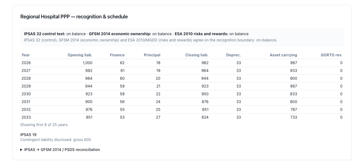
Figure 5.2 — Recognition and schedule panel for the hospital: the three boundaries on one line — IPSAS 32 control test on balance sheet, GFSM 2014 economic ownership on balance sheet, ESA 2010 risks and rewards on balance sheet —, the calculation's sentence below, and the first eight of the twenty‑five rows, with the liability opening at 1,000 and the first year's finance charge at 62, which is §4's solved rate of 6.2374%. (Steps 0 to 5.) [note: the screen does not print the rate: it is read off the first row (62.37 on 1,000.00), and amounts carry no decimals. The divergence sentence prints in English on both language settings, because the calculation generates it.]
Route: …/ipsas/arrangements/new. Input: the form's five blocks. Output: the saved arrangement; the calculations pick it up on the next run. Analyst's decision: all of Step 3 and Step 4, Step 1's three checkboxes and Step 2's eight entries.
The five blocks, with the label the screen prints:
The five fields that decide the most and are worst understood, and that §5 has to name:
Limits. (i) The contract's guarantees are not edited here: the form carries them over intact on save — so it never loses them — and reads them to derive the minimum‑revenue guarantee flag, but offers no place to write them. They only come in with the demonstration pack or by program [to be built]. (ii) There are no fields for the reclassification of own assets or for a non‑repayable grant, so rules (c) and (d) of Step 3 cannot be expressed and the initial liability is always equal to the asset [to be built]. And a naming trap the manual has to state: the fraction of capex funded by the grantor is an input to Step 2's classification and does not reduce the liability. (iii) There are no fields for the imputed loan's three entries from Step 9 — rate, term and redemption profile —, so the imputed loan is always measured with the default conventions [to be built]. (iv) There is no field for the indexation unit from Step 10.
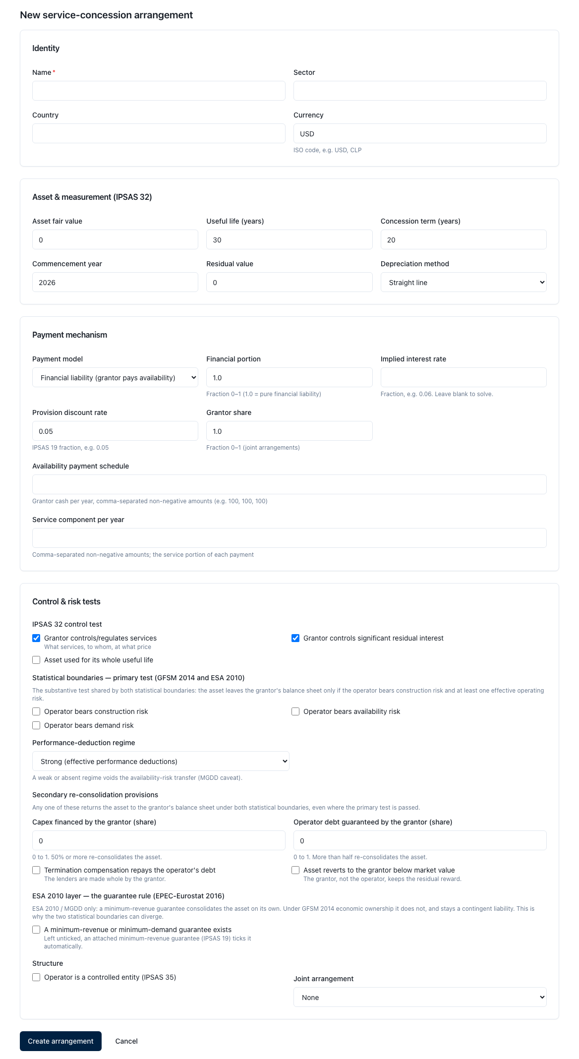
Figure 5.3 — Creation form with the five blocks and the whole of the fourth in view: the IPSAS 32 control test with its three checkboxes, the statistical boundaries — primary test with the three risk checkboxes and the deduction‑regime selector —, the secondary re‑consolidation provisions with their two fractions and two checkboxes, and the ESA 2010 layer — guarantee rule (EPEC‑Eurostat 2016). (Steps 0, 2, 3 and 4.) [note: the five blocks are five headings, not five cards: the screen groups them into four cards and the fifth — Structure — is the last sub‑block of the fourth. Nothing collapses: the form opens whole, so "the fourth expanded" describes the figure's framing and not a user action. Two of the control test's three checkboxes come ticked by default.]
Routes: …/ipsas/arrangements/<arrangement>. Input: none additional; it recalculates the saved arrangement. Output: the same creation form, now populated, plus the reconciliation panel, which is the module's densest screen and the one that runs the method's final chapter. Analyst's decision: editing the arrangement.
The panel publishes, in this order:
The three boundaries, each with its label and its outcome — "on the grantor's balance sheet" or "off the grantor's balance sheet" —, followed by two separate verdicts: whether the accounting and IMF boundaries coincide, and whether the two statistical ones coincide with each other, the latter with the reason named ("EPEC–Eurostat guarantee rule") when they do not.
The recognition schedule, with the same eight columns and the same eight‑row cutoff as the home screen.
The guarantee classification, with the provision recognized at its present value and the contingent liability disclosed at its gross exposure.
The balances bridge, as an itemized table in Spanish, with the ten line items of §3, 9.1 in their order — carrying amount, less unearned revenue, financial liability at amortized cost, perimeter difference against each boundary, imputed loan of each boundary, imputed debt of each boundary and the difference between the two — and with the measurement date in the header.
The imputed‑loan block, when there is one to measure: its opening amount labelled "capital value of the consolidated asset," its balance as of the date, its rate, its term, its redemption profile, which boundaries it applies to, its measurement basis, its declared Austral conventions and its sources. It is the only surface in the product that publishes its conventions alongside the figure, and it is the standard §3, convention (iv), calls for.
The result bridge on three bases, one column per basis — period flow, accumulated to date, full life —, with the years each one covers, and below it the date statement and the methodological note.
The measurement date is asked for now, and it was §5's most consequential limit. Since the 26‑09‑2026 integration (P13) the panel opens with a Reporting year field and a Measure button: left blank, measurement is at initial recognition; with a year, both bridges are cut on that same date and the result bridge publishes its three bases. And the screen does not leave the reader to infer what the date means — it prints the convention next to it: "As at 2031" is five complete periods since inception 2026, i.e. the close of 2030, with a third variant for when the schedule ends first and the position is measured at an earlier close. It is §3, 8.2's convention, published beside the figure.
Limits. (i) The panel's methodological texts print in English, because the calculation generates them and the screen passes them through as is: each bridge's note, the date statement, the reason for each of the three boundaries, the divergence sentence, and the imputed loan's measurement basis with its conventions and its sources [to be corrected]. In the Spanish interface the labels the screen itself supplies — block titles, both bridges' line items, the three bases — have been in Spanish since the same integration; the texts have not. (ii) One line item of the balances bridge — the European boundary's imputed loan — prints the calculation's field name, add_imputed_statistical_loan_esa2010, because the screen's label map has the IMF row and not the European one; it is the row that matters most on the toll highway, which is where that debt appears [to be corrected]. (iii) The imputed‑loan block publishes its rate, its term and its profile but not the instalment (97.58 on the highway), which the calculation does return, and writes the profile with the calculation's value (constant_annuity) instead of "level annuity" [to be corrected]. (iv) Both bridges' amounts carry no decimals, so §4's 1,500.00 reads "USD 1,500" [to be corrected]. (v) Nor does the screen ask for gross domestic product, so the panel does not publish percentages.
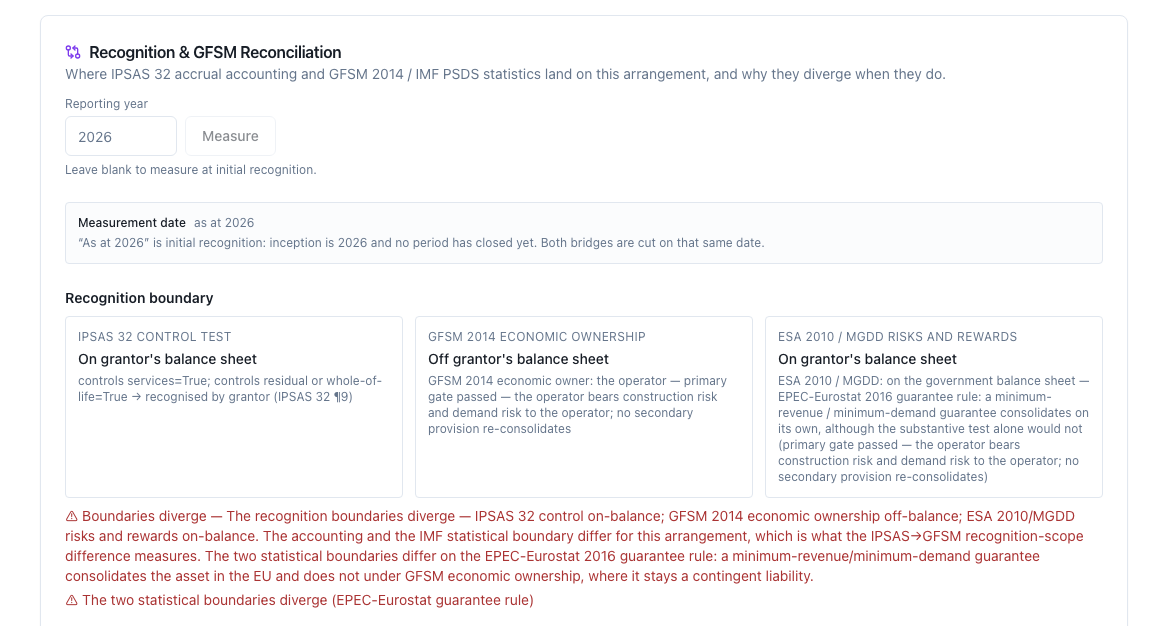
Figure 5.4 — The toll highway's three boundaries, with the Reporting year field blank and the measurement date declared as at 2026: IPSAS 32 control test on the grantor's balance sheet, GFSM 2014 economic ownership off, ESA 2010 / MGDD risks and rewards on the balance sheet under the EPEC‑Eurostat guarantee rule — and both divergence verdicts lit up, the one between the accounting and the statistical boundary and the one between the two statistical boundaries. (Steps 1, 2 and 9.) [note: each boundary's reason and the divergence sentence arrive from the calculation in English (limit (i)).]
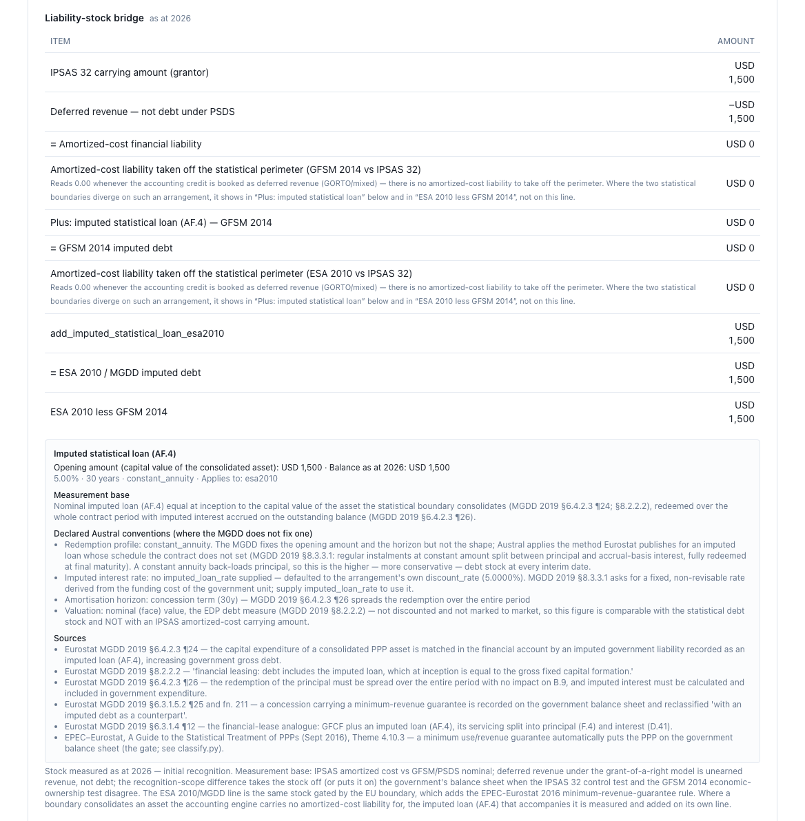
Figure 5.5 — The toll highway's balances bridge at initial recognition: IPSAS 32 carrying amount of 1,500, less the deferred revenue that is not debt under PSDS, amortized‑cost financial liability 0, GFSM 2014 imputed debt of 0 against ESA 2010 / MGDD imputed debt of 1,500 — the entire difference between the two statistical boundaries —, and below it the imputed‑loan block: capital value 1,500, rate 5.00%, term 30 years, level‑annuity profile, with its measurement base, its declared Austral conventions and its six sources from the MGDD and EPEC‑Eurostat. (Step 9.) [note: three things the draft caption asked for and the screen does not give. The 97.58 instalment from §4 is not printed — the calculation returns it and the block publishes rate, term and profile, not the instalment —; the profile comes out as constant_annuity; and amounts carry no decimals, so "1,500.00" reads "USD 1,500". And the European imputed‑debt line prints add_imputed_statistical_loan_esa2010 instead of its label, which is limit (ii) and is visible in this figure.]
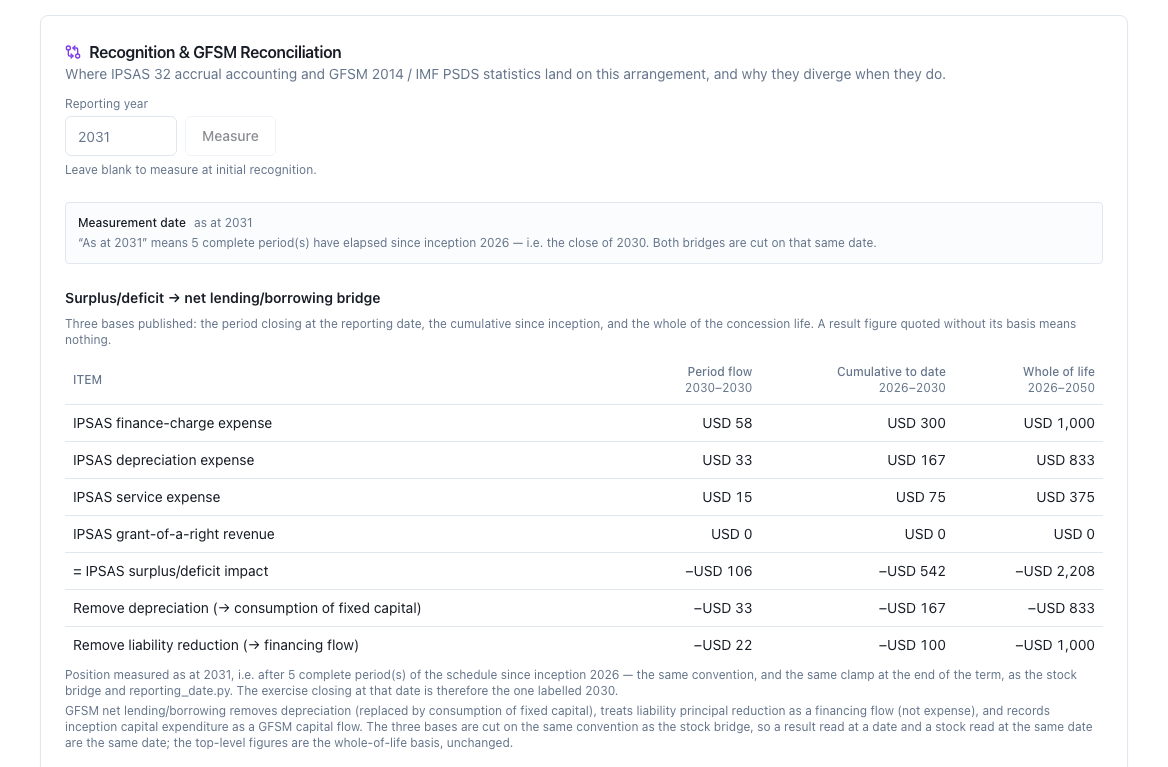
Figure 5.6 — The hospital's result bridge with the Reporting year set to 2031: the measurement date declared with its convention — five complete periods since inception 2026, i.e. the close of 2030 — and the three bases side by side with the years each one covers: period flow 2030–2030, accumulated to date 2026–2030 and whole of life 2026–2050. Finance charge 58 / 300 / 1,000; depreciation 33 / 167 / 833; IPSAS surplus/deficit impact −106 / −542 / −2,208. (Step 9.) [note: for framing, this figure hides the intervening blocks of the same screen — the boundaries, the schedule, the guarantees and the balances bridge —, which are figures 5.4 and 5.5 on the other arrangement. The two footnotes arrive from the calculation in English and one of them exposes a program route to the user (reporting_date.py), which is what §5.9's last row asks to remove.]
Route: …/ipsas/statements. Input: gross domestic product, typed in. Output: the statement of financial position with assets, liabilities, net assets, the amount attributable to government and the non‑controlling interest, with the percentage of GDP next to the three totals; the statement of financial performance with revenue, expenses and net operating result; the notes; and the disclosure set, one per component standard, each with its reference and its line items. Analyst's decision: none on the screen; it is the face of the statements.
The articulation is well resolved, and it is the first thing worth pointing out. The two faces are drawn as of the close of the same period — the first projected period of each component — and the first note says so with its year: the position is "as at" the period's close and the performance statement reports that same period, so the balances are net of depreciation, of liability amortization and of the period's unearned‑revenue release. It is exactly §3, 8.1's rule, and it is the one real packages break.
On the demonstration portfolio at first close: concession assets 5,542.02; concession liabilities 5,552.80 plus provisions 70.00, total 5,622.80; net assets −80.78. Grant‑of‑a‑right revenue 85.71; expenses — depreciation 157.98, finance charges 142.52 and provision recognized 70.00; net operating result −284.78. And a contingent liability disclosed at 600 gross.
The disclosure set carries seven notes: basis of preparation, significant accounting policies, service concession arrangements, provisions, contingent liabilities, net assets and non‑controlling interest, and commitments and subsequent events — the last one with the honest warning that the module does not capture these automatically and they must be completed from the entity's records before publication.
The provisions note now cites what supports what it states. The 26‑09 integration (P17) rewrote the note that goes to the auditor: today it attributes probability to ¶31, reliable measurement to ¶22, best estimate to ¶44, present value to ¶53, unwinding to ¶54 and its separate disclosure to ¶55 and ¶97(e) — and declares in so many words that the accrual cap is an Austral convention and not an IPSAS 19 requirement, derived from reading ¶44, ¶51 and ¶53 together, with the reason. And it closes by saying that when the undiscounted amount did not arrive with the provision the cap is not known and the balance stays flat at the recognized amount, instead of presenting that balance as if it had been measured. It is exactly what §2.4 of this manual verified, and it is the note §5 asked for before screenshotting. It is also the only one of the seven notes the module holds in both languages: a Spanish reader gets it in Spanish, and the other six arrive in the calculation's English.
Limits. (i) The face lines and the other six notes' text print in English, because the calculation generates them and the screen shows them as is: a Spanish‑reading user reads "Service concession assets" and "Provisions on concession guarantees" on the face of the statements and six of the seven notes in English [to be corrected]. It is the limit that most contradicts the series' rule — the manual must not tell the reader a different word from the one on the screen — and it is a label‑mapping fix, not a calculation change. (ii) The screen has no download button for the disclosure package (§5.8). (iii) Pensions and properties do not enter these statements from their own screens: they are aggregated only by program, and the screen's subtitle admits it — in a text that additionally exposes a program route to the user [to be corrected]. (iv) Amounts carry no decimals: §4's 5,542.02 reads "5,542" and the −80.78 reads "-81", with a hyphen and not a minus sign [to be corrected]; and in the Spanish interface the percentage of product is written with a decimal point ("9.2% del PIB") [to be corrected].
And one scope warning that belongs here, because it decides the figure's numbers. These statements also aggregate the workspace's public‑enterprise portfolio, which the screen pulls on its own from the public‑enterprise fiscal risk module. The figures above — and §4's — are those of a workspace with the concession portfolio and with no public‑enterprise portfolio. With the public‑enterprise demonstration portfolio loaded, the same screen publishes 22,582 of assets, 17,423 of liabilities and +5,159 of net assets, and the headline changes sign. It is not a defect: it is the perimeter the screen declares in its subtitle. But a reader reproducing §4 has to know what was loaded in the workspace.
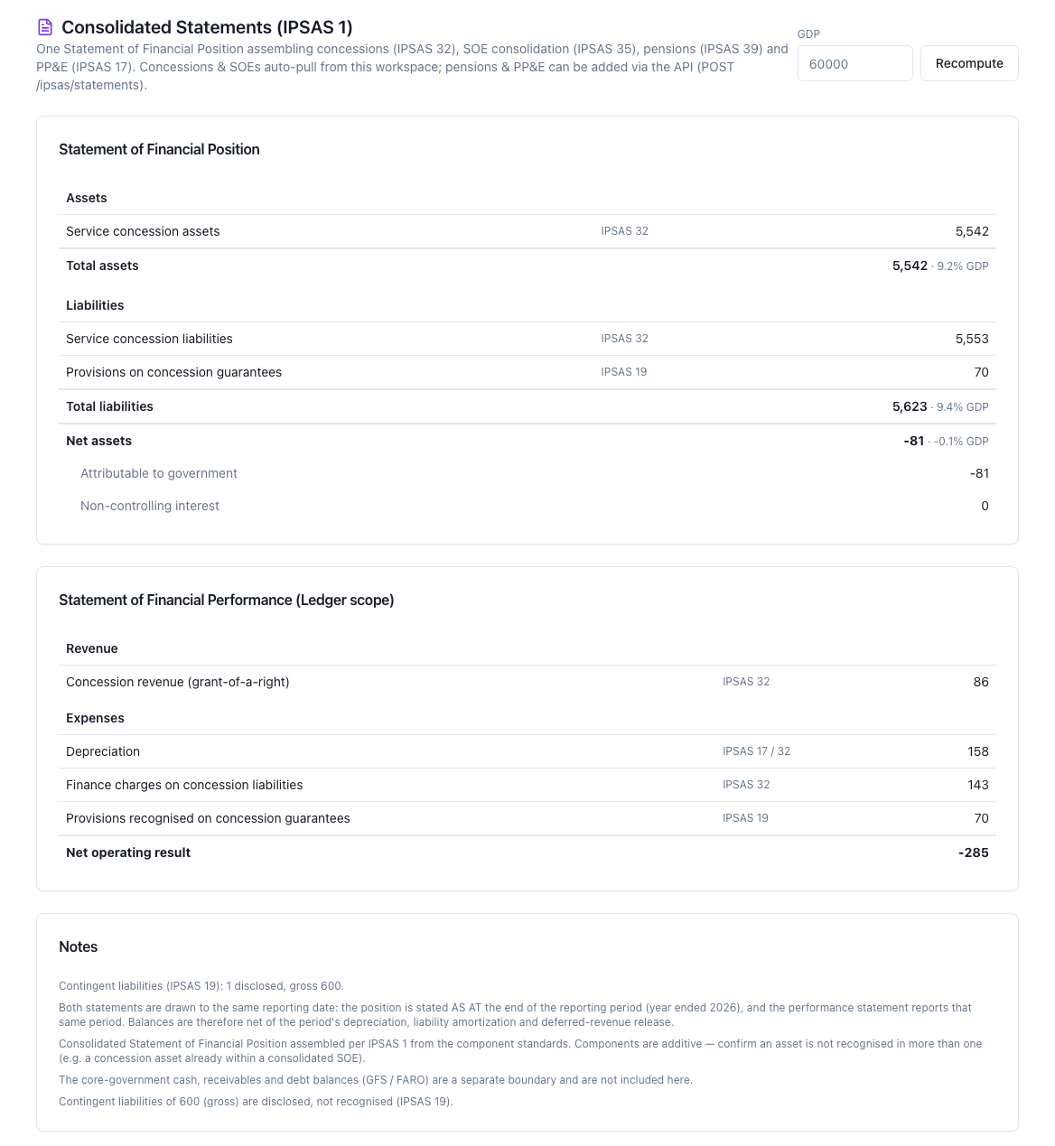
Figure 5.7 — Statement of financial position and statement of financial performance at first close: concession assets 5,542 (9.2% of product), concession liabilities 5,553 plus provisions 70, total 5,623 (9.4%), net assets −81 (−0.1%); grant‑of‑a‑right revenue 86 and expenses of depreciation 158, finance charges 143 and provision recognised 70, with a net operating result of −285. At the foot, the notes: the 600 contingent liability disclosed and not recognised, and the statement that both faces are drawn at the close of the same period. Declared product: 60,000. (Step 8.) [note: the figures are §4's (5,542.02 / 5,552.80 / 70.00 / 5,622.80 / −80.78 / 85.71 / 157.98 / 142.52), rounded by the screen to zero decimals. The face lines and four of this block's five notes are in English (limit (i)). The workspace had no public‑enterprise portfolio loaded when this figure was taken.]
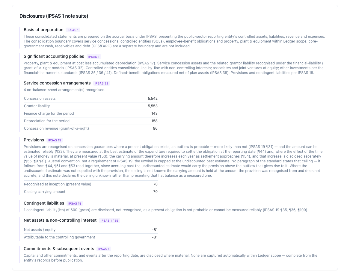
Figure 5.8 — The disclosure set: the seven notes by component standard — basis of preparation, significant accounting policies, service concession arrangements, provisions, contingent liabilities, net assets and non‑controlling interest, and commitments and subsequent events —, each with its reference and its line items. The Provisions note is the one rewritten in the 26‑09 integration: it cites only verified paragraphs, declares the accrual cap an Austral convention, and publishes the balance at 70.00 at recognition and 70.00 at close. The last note warns that the module does not capture commitments or subsequent events and that they must be completed from the entity's records. (Step 8.) [note: on the English setting the seven notes read in English, which is the calculation's own language; the provisions note is the only one the module also holds in Spanish, and the Spanish edition's figure shows it in Spanish. The contingent‑liabilities note today cites ¶35, ¶36 and ¶100.]
Route: …/ipsas/consolidation. Input: gross domestic product. Output: the consolidated position of the public‑enterprise sector — assets, liabilities, net assets with their percentage of GDP, the amount attributable to government, the non‑controlling interest and eliminated intragroup loans — and the entity table with classification, perimeter, ownership share, treatment, assets and liabilities incorporated, non‑controlling interest and the value of the interest. Analyst's decision: none here; they are decided by M6's diagnostic, and this screen consumes them.
It is taught only once and for a reason of method: it is the destination of Step 0's cut 0.3 and the boundary with M6. The public‑enterprise portfolio enters through the consolidation standard's control test — the same one M6's diagnostic prints, so the two surfaces cannot disagree about the same entity —, and at the bottom the screen states which test decides each column: classification is the 50% test from the government finance statistics manual, and perimeter is the consolidation standard's control test. Verified on screen on 28‑09‑2026: the note today cites GFSM 2014 ¶2.69 for the 50% test and IPSAS 35 for the perimeter; the correction that was pending has been integrated.
On the Spanish setting this screen is almost entirely in Spanish. What is not: the word "workspace" in its subtitle, and the calculation's warnings at the head of the screen — the one explaining that the 300 of intra‑group on‑lending is retained in consolidated liabilities because in this perimeter it is owed to the external core government, and the one warning that the broadcasting corporation fails the 50% test and is sectorized within general government. Both are warnings of method, not of system, and both arrive in English [to be corrected].
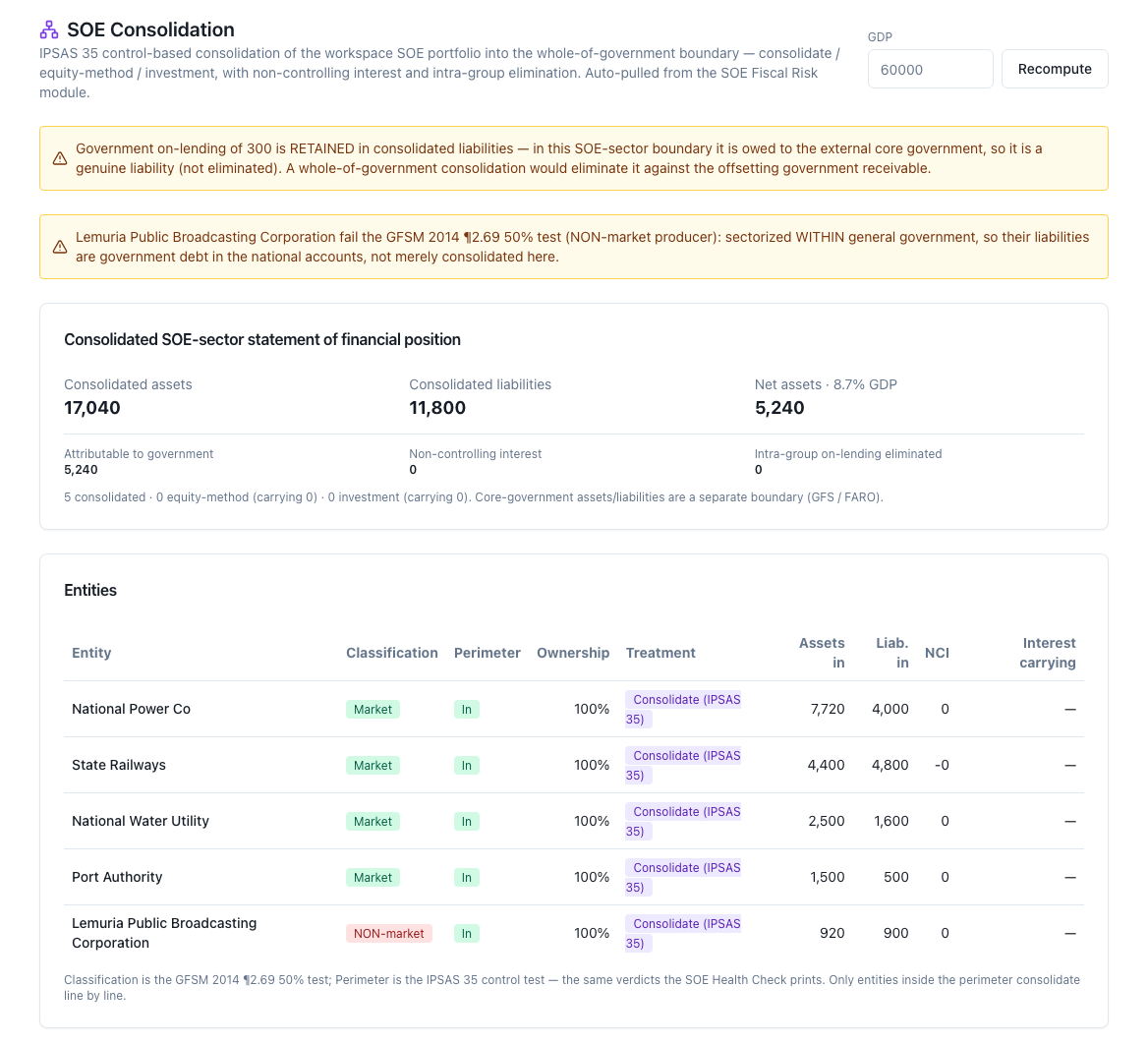
Figure 5.9 — Public‑enterprise consolidation: the five‑enterprise demonstration portfolio entering through the IPSAS 35 control test — consolidated assets 17,040, liabilities 11,800, net assets 5,240 (8.7% of product), all attributable to government, non‑controlling interest 0 —, and the entity table with its classification (the GFSM 2014 ¶2.69 50% test: four market producers, the broadcaster non‑market) and its perimeter (the IPSAS 35 control test: all five inside). At the foot, the note stating which test decides each column. (Step 0, cut 0.3.) [note: the intra‑group on‑lending eliminated line reads 0, and the warning above explains why: in this public‑enterprise‑sector perimeter the government's 300 of on‑lending is owed to an external third party and is a genuine liability; it would be eliminated in a whole‑of‑government consolidation. The railway's non‑controlling interest prints as "-0". Both warnings are in English.]
Route: …/ipsas/manual. It is the method's summary inside the product, in Spanish and in English, with two worked examples whose figures regenerate from the calculation itself and are pinned by a test, so they cannot silently drift. This manual is its extended version, not its replacement. It is named and not captured.
Three outdated points that need aligning once §3 and §5 are approved, as was done with the wave‑1 modules: (i) it declares the full presentation set from the presentation standard deferred, when the consolidated‑statements screen with its note set is in production; (ii) it describes one risks‑and‑rewards test fusing the IMF's and Eurostat's, when the module has published three separate boundaries since the band‑A correction; (iii) it says the arrangement register is administered by program, when there are creation and edit screens. Point (iv) of that list — the arrangement's split attributed to a paragraph §2 verified deals with another matter — has been closed in the 26‑09 integration: the on‑screen manual today cites ¶27–¶28 and ¶AG50, which is what §2.2 does. The first three remain open, verified on screen on 28‑09: the manual declares the full IPSAS 1 presentation suite deferred, describes one fused GFSM/ESA risks‑and‑rewards test, and says the arrangement register is administered through the API. And the texts still use the calculation's field names in user‑facing prose (financial_portion), which the series' external vocabulary does not allow.
It is a value typed on the screen, separately on the module's home screen and on the consolidated statements — it is not read from the workspace's settings, and the two screens do not share it. [to be corrected]: as long as GDP is a screen value and not a workspace setting, nothing guarantees the two hold the same figure, and the reader has to check it on each one. And the demonstration pack still does not declare scale or source (H18): the five arrangements are in dollars with no statement of the unit.
Consequence for this manual, and it is a drafting rule from §4: every "percentage of GDP" figure carries the declared GDP alongside it, as the example's assumption and not as data. It is a rule that survives the fix: a percentage with no denominator is not verifiable even when the denominator is correctly entered.
Five conventions of the calculation the screen does not declare and the manual does, each with its effect on the example.
(1) The initial liability is always equal to the recognized asset. No exception and no field to depart from it. It is Step 3's rule (b) and it is correct; what is missing are rules (c) and (d), and the consequence is that an arrangement with a non‑repayable state grant or with a reclassification of own assets overstates the liability.
(2) The rate is solved by bisection over the interval from zero to one, with one hundred iterations and a tolerance of one millionth on the closing balance, against the payment schedule net of service. When the net payments are not enough to repay the principal, the calculation returns a zero rate with a warning instead of a made‑up number.
(3) An imposed rate that does not close the liability produces a warning with three figures: the residual, its percentage of the initial liability and the rate that does close it, to four decimal places. The warning's threshold is half a percent of the initial liability, and it is an Austral convention: loose enough for a rate rounded to two decimal points as a percentage to pass, tight enough for a materially wrong one to be flagged.
(4) The provision's accrual cap is read from a single rule, and when the balance is not known it does not accrue. Integrated on 26‑09‑2026 and verified on screen on 28‑09 (figures 5.7 and 5.8). The two routes that measure a provision — the consolidated statement's face and the point‑in‑time valuation — applied the cap with different criteria and published two amounts for the same provision at the same close; they now read the same rule and publish 70.00, which is what the consolidated statement prints both on the face and in the provisions note. The convention that rule implements is Step 7's: when the undiscounted amount did not arrive with the provision, the cap is not known, the balance stays at the amount at which it was recognized, and the note declares the cap unknown, instead of assuming the present value is the cap. A provision that does bring its undiscounted amount accrues up to it.
(5) The on‑screen schedule cuts off at eight rows and the note says so; the rest of the schedule, the postings and the post‑term depreciation exist in the calculation and on no screen.
It exists, it works, and it has no screen. It is the function that turns the module into something usable for an annual close: it restates, as of a chosen date, the arrangement's financial liability and each of its provisions, with §3, 8.2's full form — opening balance, discount unwinding, remeasurement, settled, closing balance — and one line per period. It accepts, per provision, the period's remeasurement and settled amount, and optionally a remeasurement of the financial liability; it rejects a date earlier than the arrangement's start instead of returning a meaningless figure; and it measures Step 9's bridge as of the same date, so the two artifacts of a single answer cannot disagree about the day.
Following the series' convention, what is described here is the program call in prose, and no screen is invented: the arrangement, the reporting year and, where applicable, the per‑guarantee remeasurements and settlements are passed to it, and it returns the position as of that date. On the hospital from §4: 1,000.00 at initial recognition, 900.17 as of 2031, 765.07 as of 2036 and 0.00 as of 2051 — always with §3, 8.2's convention, that "as of 2031" is the balance after five complete periods, that is, the 2030 close.
Two limits. [to be built] it has no screen, and it is the method's most accounting‑driven step. [to be corrected] it does not restate unearned revenue: for the toll highway it returns 0.00 as of 2026, 2031 and 2056, while unearned revenue runs from 1,500 to 1,250 and to zero. The position as of the reporting date for a toll concession says nothing about the one liability that concession has.
Today it works in two directions. M6's public‑enterprise portfolio feeds the consolidation through control, with the same perimeter test M6's diagnostic prints. And each arrangement's provisions and disclosures flow out to M9's consolidated fiscal‑risk register, as line items in the explicit‑contingent family: the provision with its expected cost and its provisioned flag, the disclosure with its gross exposure.
And the recognized direct liability deliberately does not flow out. It is §1.2's no‑duplication rule implemented in the right direction: the commitments register in M2 already has that line, and emitting it from here would count it twice. The calculation declares it in its own comment, and §5 repeats it because it is the kind of decision that gets lost when nobody writes it down.
What is missing. [to be built] there is no handoff from M2's commitments register to the accounting arrangement: the same contract is loaded twice, in two modules, with two data sets nobody reconciles. And [to be built] there is no handoff to the fiscal‑statistics module's statistical figure for the same project: Step 9's bridge today publishes the imputed statistical side — the band‑A correction — and accepts, as a reference line, an external figure that no caller passes it. Feeding it requires the same contract to exist in both modules, and that is product work.
The living list, as of this edition's close. Each point with what the analyst does in the meantime.
| # | Limit | What the analyst does in the meantime |
|---|---|---|
| 1 | The home screen's bridge prints unformatted, with the calculation's keys in a code block; the readable version and the measurement date are only on the edit screen | reads the bridge on the arrangement edit screen (figures 5.5 and 5.6), where the Reporting year field cuts both bridges on the same date (P13, integrated) |
| 2 | The schedule does not show unearned revenue or the service component | reads the unearned‑revenue balance off the face of the consolidated statement and the service component from its own input |
| 3 | Post‑term depreciation is calculated and not reported — 1,241.67 out of 5,700 in the demonstration portfolio, 21.8% | calculates the tail with the useful life and the carrying amount at handover, which the calculation does publish |
| 4 | The undiscounted amount for guarantees does not arrive from the risk tool, so the accrual cap is not known and the provision stays flat at the recognized amount (70.00) | reads the balance for what it is — a recognized amount with no cap measured, declared as such in figure 5.8's note — and requests the undiscounted amount from the risk tool, which is the definitive fix. The cap with two criteria on two routes, which also published 73.50 on one of them, has been closed (P11) and integrated on 26‑09 |
| 5 | The point‑in‑time valuation has no screen and does not restate unearned revenue | by program, and adds the schedule's unearned revenue by hand |
| 6 | Guarantees cannot be created or edited in the interface | loads them by program, or works over the demonstration pack |
| 7 | The disclosure package has no button and does not include the schedule, the postings or the bridge; nor is there a PDF version | obtains it by program and completes the three missing artifacts by hand (§5.8) |
| 8 | The postings are not shown on any screen, and the schedule cuts off at eight rows | by program |
| 9 | No reclassification of own assets or non‑repayable grant; the liability is always equal to the asset | adjusts outside the register and declares it in the note |
| 10 | No imputed‑loan fields (rate, term, profile) | accepts the default conventions, which the result publishes |
| 11 | No indexation, no remeasurement on modification and no impairment — and every Chilean concession is denominated in unidad de fomento | runs Step 10 entirely outside the tool |
| 12 | An arrangement with no payment schedule dates its start at year zero and publishes an absurd number of periods | avoids loading an arrangement with only guarantees, or corrects the metadata by hand |
| 13 | The consolidated statements' lines and six of their seven notes, the consolidation's warnings and the bridges' methodological texts print in English (the bridge labels and the provisions note have been in Spanish since 26‑09) | translates them when preparing the package |
| 14 | The three result screens print amounts with no decimals, so no §4 figure can be read on screen with its two decimal places, and the percentage of product uses a decimal point on the Spanish interface | cites §4 for the decimals, and reads the screen as confirmation of the order of magnitude |
| 15 | Pensions and properties do not enter the consolidated statements from their screens | by program, if the scope calls for it (outside this manual) |
| 16 | The demonstration pack has no country, scale or source, and GDP is an interface value | publishes the declared GDP alongside each percentage |
| 17 | Several user‑facing labels depart from the official terminology in Spanish (§5.9) | uses the manual's terminology and requests the fix |
| 18 | The pure shadow toll has no expression: the financial‑liability model with a schedule recognizes a liability, and there is no way to declare usage‑based payments with no unconditional obligation | leaves the schedule empty and carries the payments outside the register, with the note |
| 19 | The control test's written rationale and the instrument backing each of Step 2's fractions have no field | keeps them in the evidence folder and cites them in the note (it is the method's largest audit gap) |
| 20 | One line item of the balances bridge prints the calculation's field name (add_imputed_statistical_loan_esa2010) instead of its label, and it is the row where the toll highway's European imputed debt appears |
reads it by its position — it sits between the European scope difference and the European imputed debt — and requests the missing label |
| 21 | The on‑screen manual still declares deferred the presentation set that is already built, describes one fused GFSM/ESA risks‑and‑rewards test where the module publishes three boundaries, and says the arrangement register is administered through the API where there are creation and edit screens | ignores it and refers to §5.2 |
| 22 | The imputed loan's annual instalment (97.58) is not published alongside its rate, its term and its profile, although the calculation returns it, and the profile prints with the calculation's value (constant_annuity) |
takes the instalment from §4 and the profile from the declared conventions, which are printed |
And one thing the module does well and is worth stating, because it is §6's counterexample: above the sixty‑arrangement cap the portfolio calculations refuse to run instead of truncating the list. A spreadsheet sums whatever fits in its range.
It is the file an accountant takes to the comptroller's office or to the external auditor, and today it exists in a single format — spreadsheet — with four sheets: statement of financial position, statement of financial performance, recognition by arrangement and notes and disclosures. It accepts Spanish or English as the language, and gross domestic product; the file name carries the language; the amounts go to two decimal places, deliberately, because at zero decimal places the printed totals did not square.
The recognition sheet is the most useful one and the one that comes closest to the module's headline: one row per arrangement with recognition, control test, the two statistical boundaries kept separate, liability model, initial asset and liability, and two divergence columns — accounting against the IMF, and the two statistical ones against each other — computed over the boolean results and not over the sentence's text, which is what used to flag divergence on every row.
What it lacks, and it is a lot for an audit package. [to be built]: it has no download button on any screen — the module's deliverable is unreachable from the product and is only obtained by program. And it does not include the year‑by‑year amortized‑cost schedule, the double‑entry postings or the bridge to the statistical figure, which are the three artifacts that set this module apart from any ordinary financial statement, and the third is the one its own method calls the flagship deliverable. Nor is there a PDF package.
And a language warning that degrades the Spanish‑language package: the language setting localizes the sheet names, the statement titles, the section and column headers and the result‑cell labels, and not the statement lines, which arrive from the calculation in English. A package requested in Spanish arrives with its headers in Spanish and its line items in English [to be corrected].

Figure 5.10 — The Recognition (IPSAS 32) sheet of the disclosure package: one row per arrangement with recognition, control test, the two statistical boundaries kept separate, liability model, initial asset and liability and the two divergence columns. The toll highway is the only row that flags "Yes" in both; the other four flag "No" in both. Amounts go to two decimal places (1,500.00), which is the only surface in the module where §4 can be read with its decimals. (§5.8.) [note: the package has no button and was obtained by program (limit 7), over the same portfolio and the same workspace as figures 5.1 to 5.8. The figure is the sheet exactly as it comes out of the workbook. The Spanish edition of this manual carries the Spanish package in the same figure, where the language warning of the paragraph above is visible: the headers are in Spanish and the values — grantor_asset, financial_liability, grant_of_a_right — arrive from the calculation in English. Two headers are cut off by the workbook's own column widths.]
It is the series' rule, and here it has a concrete list, because the module does not say the same thing to itself. The correction §5 treated as pending was integrated on 26‑09‑2026 and resolved a part of it; the list below is re‑verified screen by screen on 28‑09.
What that correction resolved, and what this manual already writes in its official form: la concedente in the feminine, carga financiera ("finance charge") instead of cargo financiero, importe en libros ("carrying amount") instead of valor libro, concesión de un derecho al operador ("grant of a right to the operator"), and base contable de acumulación (o devengo) ("accrual basis of accounting"). Added to them: SEC 2010 on the home screen, in the form and in the portfolio badge, and prueba de control de la IPSAS 32 in the form.
What remains open, verified in production on 28‑09‑2026 [to be corrected]:
| Concept | What the product prints | Official form |
|---|---|---|
| arrangement | «arreglo» on the home screen («Nuevo arreglo», «Arreglos», «Arreglo» — "New arrangement," "Arrangements," "Arrangement") and in the creation title | acuerdo (the standard's title in Spanish is Acuerdos de Concesión de Servicios, "Service Concession Arrangements") |
| grant‑of‑a‑right revenue | «Ingreso GORTO», an untranslated English acronym in a column header | ingreso por concesión de un derecho ("grant‑of‑a‑right revenue") |
| finance charge (schedule column on the home screen) | «Financiero» | carga financiera |
| carrying amount (schedule column on the home screen) | «Valor libro del activo» — while the edit screen of the same module already says «Importe en libros del activo» | importe en libros del activo |
| reconciliation | «Reconciliación» on the edit screen | conciliación |
| control test | «Test de control» on the edit screen | prueba de control (which is what the home screen calls it) |
| ESA 2010 | half resolved, and worse than before: the home screen now says «Riesgos y beneficios SEC 2010:» and the badge «SEC ≠ GFSM», and the form «Capa SEC 2010»; the edit screen still says «Riesgos y beneficios ESA 2010 / MGDD», «Deuda imputada ESA 2010 / MGDD» and «ESA 2010 menos GFSM 2014», and the Spanish disclosure package still labels its columns «ESA 2010 en balance» and «ESA≠GFSM» | SEC 2010 and «SEC ≠ GFSM» on all three surfaces, which is the Spanish form and the one this manual's §2 uses in its eight occurrences (in the English edition, «ESA 2010» is correct) |
| boundary (portfolio column) | «Límite» | frontera, which is what the rest of the module and all of this manual call it |
| liability model (portfolio column) | «financial liability», «grant of a right», «mixed» — the calculation's own value, untranslated, in a column of a Spanish table | pasivo financiero, concesión de un derecho, mixto, which is what the form's own selector calls them |
| amortisation profile (imputed loan) | constant_annuity |
anualidad constante ("level annuity") |
| — | add_imputed_statistical_loan_esa2010, the calculation's field name printed as the label of a balances‑bridge line item (on both language settings) |
Más: préstamo imputado estadístico (AF.4) — SEC 2010, which is the label its IMF twin row already has |
| — | «workspace», «PP&E» and two program routes in user‑facing text: POST /ipsas/statements in the consolidated statements' subtitle and reporting_date.py in the result bridge's footnote |
translate them and remove the routes |
The fourth row deserves a paragraph, because it is a consistency finding and not a translation one: after the pending correction, two screens of the same module will call the same amount two different things — "Valor libro del activo" on the home screen and "Importe en libros del activo" on the arrangement edit screen — which is worse than having both wrong. The home screen's fix is the same line of work and has to be made in the same pass.
The module is tried with no registration, with the demonstration portfolio loaded from its own home screen, and everything this §5 describes can be reproduced on screen with §4's figures. The client keeps the tool and the capacity to operate it: §3's method is self‑contained and does not depend on it, and the tool runs the method without asking the user to trust a closed box — it publishes the test that decided each boundary, the rate it solved for, the basis with which it measured each provision, and the conventions it had to fix where the source fixes none.
This has to start with a concession, and it is not a courtesy. A spreadsheet develops a liability at amortized cost perfectly well. It is a second-year course exercise: a column for the opening balance, one for interest, one for payment, one for the closing balance, and the goal-seek function to solve for the rate. The Regional Hospital's schedule from §4 is twenty-five rows and five columns, and a spreadsheet calculates it and teaches it better than any screen. This manual is not written against that calculation.
This section's argument is a different one, and narrower: what happens to that calculation once it stops being a calculation and becomes the book of a portfolio. A concessions book has forty contracts that all have to close every year, three rule books that classify them differently, guarantees that arrive already valued from another unit, two clocks per contract that do not coincide, and an auditor who in three years is going to ask where a figure came from. None of those five things is a problem of arithmetic; all of them are problems of perimeter, invariants and provenance, and none is solved with a better formula.
The eight failures that follow are not hypothetical. Each is presented the same way: where it occurs (which §3 step), what fails on the spreadsheet, how much it costs, measured over Lemuria's portfolio from §4, and what the tool does instead. And two of them happened to the tool itself: they are told the same way as the rest, with their figure, because the difference between a spreadsheet and a program is not that the program never errs, but that when it errs it leaves a trace, gets corrected once for all forty contracts, and a test remains that keeps it from coming back.
Where it occurs. Step 2, and it is the failure that orders all the others.
What fails on the spreadsheet. The spreadsheet puts up a cell — "is it on the balance sheet?" — with two possible values, and with that it treats the recognition question as answered. It is not laziness: the format forces it. A cell cannot hold three answers, and whoever builds the spreadsheet has to choose which of the three rule books governs. They choose the one they are asked for that month.
How much it costs in Lemuria. The Coastal Highway admits three simultaneous, true answers:
| Boundary | At inception | At 2031 |
|---|---|---|
| IPSAS 32 — recognized asset / unearned revenue | 1,500.00 | 1,250.00 |
| GFSM 2014 — statistical debt | 0.00 | 0.00 |
| ESA 2010 / MGDD — statistical debt | 1,500.00 | 1,375.25 |
Over the whole portfolio, the highest and the lowest reading are 2,500.00 apart, 4.17% of GDP (GDP 60,000). That is the size of the error that fits inside a yes-or-no cell. And it is not a calculation error: the spreadsheet's arithmetic is done correctly. It is that two tests were missing that the spreadsheet did not know it had to run.
What the tool does. The three tests run on the same contract, under its own name, and all three are published, each with the written basis that decided it. The divergence is not resolved: it is measured, and its amount is the figure for Step 9's bridge. And a badge on the portfolio lights up the contract where the boundaries do not coincide, which is the one that has to be read carefully and the one that on a spreadsheet is indistinguishable from the rest.
Where it occurs. Steps 4 and 5, in the input.
What fails on the spreadsheet. The State pays 95.00 a year, and the spreadsheet applies it against the liability. It is the natural operation: the payment is in the contract, the liability is in the column next door. But 15.00 of that 95.00 is not debt service: it is the price of a service — cleaning, catering, maintenance — that the operator provides that year and that never formed part of the asset. Putting it into the liability books as amortization what is actually current consumption.
How much it costs in Lemuria. It depends on how the spreadsheet gets it wrong, and the two variants are instructive.
Variant (a): keeps the correct rate (6.2374%) and applies the full payment. The liability over-amortizes every year:
| Year | Correct liability | Spreadsheet liability | Difference |
|---|---|---|---|
| 2026 | 982.37 | 967.37 | 15.00 |
| 2030 | 900.17 | 815.21 | 84.96 |
| 2035 | 765.07 | 565.14 | 199.93 |
| 2040 | 582.24 | 226.72 | 355.52 |
| 2043 | 442.85 | −31.30 | 474.15 |
| 2045 | 334.82 | −231.25 | 566.07 |
The spreadsheet's liability is extinguished in 2043, seven years before the term, and it keeps going: by 2050 it reads −851.01. A negative liability of 851.01 is an asset no one has, and no spreadsheet check flags it, because the spreadsheet does not check that the liability closes at zero: it checks that it reaches zero. And the period's expense is understated by 15.00 every year — the entire service component — and by 375.00 over the life of the contract.
Variant (b): solves for the rate against the gross payment. Now the liability does close at zero, and the error hides inside the rate:
| Correct | Spreadsheet | |
|---|---|---|
| Implicit rate | 6.2374% | 8.1647% |
| Lifetime finance charge | 1,000.00 | 1,375.00 |
| Lifetime service expense | 375.00 | 0.00 |
| Maximum balance difference | — | 50.85 (5.1% of the initial liability) |
The spreadsheet reclassifies 375.00 of service expense as finance expense and pushes the implicit rate up by 1.93 percentage points. In public accounting those two lines are not interchangeable: one is the period's current consumption and the other is the cost of debt; they go to different accounts in the budget classifier, they are treated differently in the statistical bridge, and one of the two is what a debt analyst uses to estimate the sovereign's cost of financing. An implicit rate of 8.1647% published by a country that finances itself at 6.2374% is a figure that misleads whoever reads it.
What the tool does. The separation is in the input form, not in the formula: the per-year service component is its own field on the arrangement, distinct from the payment schedule, and the rate is solved against the payment net of that component. No calculation can confuse them, because they are never in the same cell. And the two lines come out separately in the results bridge, which is where it matters.
Where it occurs. Step 5.
What fails on the spreadsheet. Someone types in a rate. Not out of carelessness: because they have one on hand and it is plausible — the rate on the loan that financed the works, the social discount rate, the one used last year. The spreadsheet calculates obediently, and the liability does not close at zero. The residual sits in the last row, twenty-five rows down, where no one looks.
How much it costs in Lemuria. Over the Regional Hospital, with the same payment schedule:
| Typed-in rate | Residual at 2050 | % of the initial liability |
|---|---|---|
| 6% (the loan's) | −97.29 | −9.73% |
| 6.24% (the correct one, rounded to two decimals) | 1.11 | 0.11% |
| 6.2374% (the solved-for one) | 0.00 | 0.00% |
| 8% (social discount) | 1,000.00 | 100.00% |
| 5% (last year's) | −431.81 | −43.18% |
The 8% row is the limiting case and is worth reading. At that rate the first year's finance charge (80.00) exactly equals the net payment (80.00), so the liability never amortizes: twenty-five rows of a balance that does not move, and a residual that is the entire initial liability. A spreadsheet prints it unfazed; an accountant skimming it sees a tidy column of identical numbers and turns the page.
The 6.24% row is the other lesson: a rate rounded to two decimal points in percentage terms leaves a residual of 1.11 — 0.11% of the liability — and that is fine. Not every difference is an error, and a tool that warns over 1.11 teaches its users to ignore warnings.
What the tool does. It solves for the rate by bisection against the schedule, so the normal case has no typed-in rate. And when the user imposes one — which is legitimate: they may want to reproduce another unit's calculation — it checks the residual against a threshold of half a percent of the initial liability (5.00 on this contract) and warns when it is exceeded, with the residual and the correct rate in the warning text. The 6.24% row passes with no warning; the other three get it.
Where it occurs. Steps 4 and 6, in the grant-of-a-right model.
What fails on the spreadsheet. The Coastal Highway's credit — 1,500.00 of unearned revenue — gets entered once, in the inception year's row, and stays there for thirty years. No one releases it, because releasing a liability that no one is going to pay does not resemble any operation anyone knows. The worse variant is the one that does not even record it: "that's not debt, it doesn't go on the schedule."
How much it costs in Lemuria.
| Year | Correct balance | Spreadsheet balance | Revenue not recognized |
|---|---|---|---|
| 2026 | 1,450.00 | 1,500.00 | 50.00 |
| 2030 | 1,250.00 | 1,500.00 | 250.00 |
| 2035 | 1,000.00 | 1,500.00 | 500.00 |
| 2045 | 500.00 | 1,500.00 | 1,000.00 |
| 2055 | 0.00 | 1,500.00 | 1,500.00 |
At contract termination the spreadsheet is still carrying 1,500.00 of liability that no longer exists and has failed to recognize 1,500.00 of accumulated revenue. Two faces of the same error, and neither shows up as an imbalance: the spreadsheet's balance sheet balances perfectly every year, with a figure too high in liabilities and one too low in net assets.
The variant that omits everything is worse in one direction and better in another: it does not inflate the liability, but it erases 50.00 of revenue per year for thirty years and leaves a 1,500.00 asset with no counterpart, which is an imbalance the spreadsheet papers over by dumping it into net assets.
What the tool does. Straight-line release over the term is part of the schedule, not a manual adjustment, and the unearned revenue balance is published in the same table as the financial liability. (The schedule screen does not yet print that column — it is declared in §5 — and the balance is obtained from the full schedule. It is exactly the kind of gap this chapter objects to, and it is told no differently for being its own.)
Where it occurs. Step 6.
What fails on the spreadsheet. The spreadsheet depreciates the asset over the contract term. It is the natural shortcut: the contract runs twenty-five years, the spreadsheet has twenty-five rows, and depreciating over twenty-five makes the asset reach zero the same year the liability reaches zero. It comes out tidy. And it erases the asset the State receives.
How much it costs in Lemuria.
| Arrangement | Correct depreciation (useful life) | Spreadsheet depreciation (term) | Asset erased at handover |
|---|---|---|---|
| Regional Hospital | 33.33 | 40.00 | 166.67 |
| Coastal Highway | 37.50 | 50.00 | 375.00 |
| Metropolitan Light Rail | 57.14 | 71.43 | 400.00 |
| Airport Co-investment | 30.00 | 40.00 | 300.00 |
| Total | 1,241.67 |
1,241.67 of public asset disappears: 21.8% of what the portfolio recognized, 2.07% of GDP. And it disappears silently. The error produces no imbalance, shows up in no reconciliation and leaves no trace in the final year's statement of performance: simply, on the day the contract ends, the hospital that is still standing is on no balance sheet.
There is a second, more subtle and more costly consequence: the spreadsheet's annual depreciation is higher — 40.00 against 33.33 on the hospital — so the concession's result for each period comes out worse than it is. A State that uses that figure to decide whether concessioning is worthwhile is comparing a badly measured concession against a well-measured public works project.
What the tool does. Two independent horizons: depreciation runs over the greater of useful life and term, and the carrying amount at handover is published per contract. (The charges after termination are calculated and today are not reported in the table, because the schedule has the length of the payment calendar; it is declared in §5. The handover figure is correct; what is missing is the table's continuation.)
Where it occurs. Step 7, and it is the failure that happened to the tool itself.
What fails on the spreadsheet. Two opposite errors on the same figure, and both are natural.
The first: the guarantee's expected cost arrives already at present value from the tool that values it. The spreadsheet, which applies discounting to anything that looks like a future flow, discounts it again.
The second: a provision at present value accretes the discount every period, and that accretion has a ceiling — the undiscounted best estimate, which is an Austral convention and not a paragraph of the standard (§2.4). The spreadsheet has an accretion column and does not have the ceiling, because the ceiling requires knowing the obligation's payment horizon, and that datum usually does not come with it.
How much it costs in Lemuria. Over the highway's minimum revenue guarantee (70.00 at present value, discount rate 5%):
| Double discounting | Amount |
|---|---|
| Correct measurement (the present value received) | 70.00 |
| Discounted one more period | 66.67 |
| Discounted over the contract's whole term (30 periods) | 16.20 |
| Discount accretion | No ceiling | With the ceiling |
|---|---|---|
| 2027 | 73.50 | 70.00 |
| 2031 | 89.34 | 70.00 |
| 2036 | 114.02 | 70.00 |
| 2046 | 185.73 | 70.00 |
| 2056 | 302.54 | 70.00 |
| 2080 | 975.71 | 70.00 |
The two errors pull in opposite directions and neither offsets the other: double discounting shrinks the provision to a quarter of its value if applied over the full term, and accretion with no ceiling multiplies it by fourteen over half a century. And because they run in opposite directions, a portfolio that commits both publishes an aggregate figure that looks reasonable and that belongs to no one.
What the tool does. The provision is measured at the present value the valuation tool delivers, and the undiscounted amount is used only as the accretion's ceiling. On this portfolio that amount did not arrive, so the ceiling is not known: the balance is held at the 70.00 for which the provision was recognized, and the note that goes to the auditor declares the ceiling unknown rather than presenting the flat balance as measured. The module's two routes — the consolidated statement's face and the position at a date — read that rule from a single place and publish the same figure, pinned down by a test that compares them against each other.
And here is the lesson that matters, and it is about the spreadsheet. The ceiling rule did not come into existence all at once: for a while the module itself applied it under two different criteria in two routes that measured the same provision at the same date, and it published 73.50 by one and 70.00 by the other. It is this chapter's failure happening to a program, and that is why it is told. What distinguishes it from the spreadsheet's case is not that it did not happen: it is how long it lasted and what closed it. Two routes that diverge have one locatable cause, one correction, and a test that compares them again on every run; when two tabs diverge in a forty-tab spreadsheet, no one notices, because nothing compares one sheet with another. This chapter's argument was never that a program does not err. It is that when it errs there is one figure to correct, in one place, and something that keeps it from coming back.
Where it occurs. Step 8.
What fails on the spreadsheet. The two faces at different dates. The statement of financial position is put together with the initial recognition amounts — which are the ones written into the contract and the easiest to find — and next to it goes the period's statement of performance. No one decides it: it happens because the two sheets were built at different times and no one wrote the date in the header.
How much it costs in Lemuria.
| At inception | At the 2026 close | Difference | |
|---|---|---|---|
| Assets | 5,700.00 | 5,542.02 | 157.98 |
| Liabilities | 5,700.00 | 5,622.80 | 77.20 |
| Net assets | 0.00 | −80.78 |
The zero in the first column is spurious. It comes from subtracting a January liability from a January asset, with a December statement of performance next to it that charges 157.98 of depreciation on assets the other face has not depreciated. The 157.98 difference in the assets line is exactly that depreciation: the error is not random, it is the size of a line in the statement sitting right next to it.
And it produces the worst kind of figure: one that looks healthy. Net assets of 0.00 suggest a balanced perimeter; the true figure — −80.78 — suggests what is actually happening, which is that a concessions portfolio's first year consumes net worth. Both sentences are about the same State in the same year.
What the tool does. Every balance is taken at the close of the period whose flows the statement of performance reports: the asset at its closing carrying amount, the liability at its closing amortized balance plus the closing unearned revenue, the provision at its closing charge. And the date is written on both faces and in the first note, which is what lets someone review it.
Where it occurs. Step 9, and it is the failure that closes the chapter.
What fails on the spreadsheet. It is not a failure of the spreadsheet: it is a failure of three spreadsheets. The accounting liability is kept by the accounting office, the budget commitment is kept by the budget unit, the statistical debt is kept by the statistics office, and the guarantees' exposure is kept by the fiscal risk unit. Each is right within its own file. None has the bridge, because the bridge requires that the four figures be calculated over the same contract, as of the same date and with the same perimeter, and that is precisely what three separate files cannot guarantee.
How much it costs in Lemuria. Five figures from the same handful of contracts, all correct, as of the same day:
| Figure | Amount | % of GDP | Who publishes it |
|---|---|---|---|
| Nominal contractual commitment | 6,495.00 | 10.82% | the commitments and contingencies register |
| Liability recognized under IPSAS 32 | 5,700.00 | 9.50% | the government accounting office |
| Statistical debt under ESA 2010 / MGDD | 4,700.00 | 7.83% | no one: Lemuria does not apply that rule |
| Statistical debt under GFSM 2014 | 3,200.00 | 5.33% | the statistics office |
| Gross exposure of the contract's guarantees | 1,000.00 | 1.67% | the fiscal risk statement |
Between the first and the last there is a factor of six and a half, and all five are true. The difference between the first two — 795.00 — is not an error or an adjustment: it is the future finance charge and service component, which are committed cash and not a liability of today. The difference between the second and the fourth — 2,500.00 — is the recognition gap, and it is the number this manual is about.
What happens with no bridge is predictable and happens every year somewhere: a report adds up two of the five, or publishes the lowest without saying which one it is, or an audit discovers that the accounting office and the debt office have spent three years reporting the same contract under two different perimeters and no one had noticed, because both reports were correct.
What the tool does. A single register for the contract, and the five figures as views of the same calculation, each labelled with the rule that produces it and the date at which it is measured. Step 9's bridge publishes the full chain — carrying amount, less the unearned revenue that is not debt, plus or minus the perimeter difference, plus the imputed statistical loan — so that a reviewer can walk it line by line instead of taking the total on faith. And the rule that avoids double counting is one of nature and is implemented in that direction: to the consolidated fiscal risk register go the guarantees' provisions and disclosures, and the recognized direct liability does not go out, because that line already belongs to the commitments register and issuing it would count it twice.
Something real is lost, and it is worth saying so. A spreadsheet is better for understanding a contract. The hospital's schedule, with its five columns in plain view, teaches what amortized cost is in two minutes; a screen that shows the first eight rows of twenty-five teaches less. For thinking through a new contract, for testing a payment structure, for explaining to a budget director why the liability barely goes down in the first five years, the spreadsheet remains the right tool, and this manual recommends it for that.
Something else is gained, and it is what a book needs. That the five figures come out of the same calculation. That the three boundaries always get run, and not only when someone remembers to. That the liability closes at zero because the rate was solved for and not because it was fudged. That the unearned revenue gets released even though no one pays it. That the asset keeps existing the day after handover. That the two statements carry the same date. That the entries balance year by year across the four contracts, the 766 of them, with not a single unbalanced period — and that someone can check it. That when a rule is wrong, it is wrong once and gets corrected for the forty contracts.
The boundary between the two tools is sharp, and it is not one of size: a spreadsheet is for understanding a contract; a book is for closing a period and defending its figure to whoever audits it. §5 shows which part of that book is built today and which part is not yet.
All references were consulted on 24 September 2026. Unless stated otherwise, each document was read in its official version — the PDF downloaded from the publisher's site — and the paragraphs cited in §2 were checked one by one against that text. ✔ = verified by direct reading for this manual · ✔M2 / ✔M6 = verified for M2 or M6 of this series and not reread · ✔f = a fact or piece of content verified within another primary source read here, without directly reading the document itself · ✔RR = verified and logged with date in Austral's own paper The Recognition Rule, from which it is taken · PV = to be verified (existence confirmed; the figure cited is checked against the document before it is quoted in the body).
Source‑access rule. When the publisher's site blocks the download — a 403 code or a captcha — the reference stops there: it stays PV, goes onto the list of manual downloads at the close of this section, and the claim that depended on it is not made. The block is not circumvented by any route. A document that has simply been moved, has a broken link, or whose server is down is not a block, and in that case the correct address is sought in the publisher's own indexes or public catalogues.
(Corrects the body and contradicts Austral's own paper. §2.6 cited, via The Recognition Rule, «an off‑balance‑sheet stock of just under £35 billion, close to 2.5% of GDP, at March 2010» attributed to this report. That figure is not in this report. All 312 pages were searched: "2.5 per cent of GDP" appears not once, nor does "March 2010", and "PFI" / "Private Finance" appear on only one page, 237. What the report gives is £39 billion of capital liability recognized in the consolidated accounts against £6 billion within net debt — £33 billion off — with no date and no percentage of GDP given. The body now publishes that figure, with its page. The report also has no box on the treatment of these contracts: its only boxes are 1.1 (wider measures of the public‑sector balance sheet), 4.1 (the regulatory response to the crisis) and 10.1. The two boxes the paper links — «What if all PFI deals were brought on balance sheets?» and «Treatment of PFI contracts in National Accounts and WGA» — therefore belong to another publication of the fiscal council, and which one could not be determined: obr.uk also returns 403 on those pages and, under the access rule in the header, the block was not circumvented. A correction is still pending in the paper, not in this manual: see the notice at the close of this section.)
15. United Kingdom — HM Treasury (2024). Charter for Budget Responsibility: Autumn 2024. Published 30 October 2024. ¶3.7: the fiscal mandate is supplemented with "a target to ensure debt, defined as Public Sector Net Financial Liabilities (PSNFL), is falling as a share of the economy by 2029‑30, until 2029‑30 becomes the third year of the forecast period"; ¶3.4 lists the set of metrics the fiscal council must report on, including net debt, net debt excluding the central bank, net financial liabilities, public‑sector net worth and general government gross debt; ¶3.6 (the current‑budget rule) and ¶3.9 (suspension in an emergency). https://assets.publishing.service.gov.uk/media/678fbb377bb65baf62c2ada8/Charter_for_Budget_Responsibility_Autumn_2024_Accessible.pdf. ✔ (official PDF downloaded and read). (Added: the working index gave the October 2024 change as "to be verified"; it is now verified against the instrument that establishes it. §2.6's reading of why widening the measure does not move the recognition line is a derivation the manual makes from reference 9, §6.4.2.3 ¶24, and is stated as such in the body.)
16. United Kingdom — HM Treasury. Whole of Government Accounts. The accounting consolidation of controlled entities, where private finance initiative contracts are recognized under IFRIC 12 when the State "controls or regulates the services". ✔M2 (edition for the year ended 31 March 2023, HC 289, November 2024) · PV the edition current when this manual is published, and the exact date central government adopted international financial reporting standards, which §2.6 places in fiscal year 2009‑10 on the authority of reference 12.
17. Chile — Decreto Ley N.º 1.263, de 1975 [Decree Law No. 1,263 of 1975], Orgánico de Administración Financiera del Estado [State Financial Administration Act], art. 40, fifth to seventh subparagraphs, added by art. 18 de la Ley N.º 20.128 [Law No. 20,128] on fiscal responsibility (2006): an annual obligation to report the amount and features of State guarantees and to estimate the financial commitments that generate contingent liabilities, "such as […] guarantees granted for infrastructure concessions". ✔M2 (text read in both instruments for that manual).
18. Chile — Budget Office (DIPRES), Chile's Ministry of Finance. Informe de Pasivos Contingentes [Contingent Liabilities Report]. The disclosure practice: the concessions system's minimum revenue guarantee reported as a contingent liability, with its maximum exposure and its expected value estimated by simulation, and the concessions system's disputes as a separate line. ✔M6 (2025 edition, December 2025) and ✔RR. The structure and method are cited; no client figures are used and no contracts are named in this section.
19. Chile — Contraloría General de la República [Office of the Comptroller General], Resolution No. 1, of 19 January 2026 (enacted 19‑01‑2026, published in the Official Gazette on 11‑02‑2026; extracted text on Ley Chile, accessed 26‑09‑2026): approves the Rules Governing the National General Accounting System for the Public and Municipal Sector under an "indirect adoption of IPSAS" — a national standard built on the 2022 Handbook of International Public Sector Accounting Pronouncements (reference 4b) — mandatory from 1 January 2027 for central government, all regional governments and all municipalities (with their incorporated services, corporations and foundations), and which from that date repeals CGR Resolutions No. 16 of 2015 and No. 3 of 2020, and Official Letter No. 11,061 of 2020 on the municipal chart of accounts (arts. 1‑2, p. 2 of the extract). ✔ the standard in force and the timetable, by direct reading of the official extract. PV the specific treatment the Rules give to service concession arrangements: the available extract carries only the repealing and effective‑date resolve, not the full text of the Rules approved under art. 1, which is cited by its full text on contraloria.cl. The Chile row of table 2.6 is corrected to the level this verification allows: the regime and the timetable, not the accounting treatment of the concession.
20. Chile — concession of the Camino Internacional Ruta 60 Ch [the Ruta 60 Ch International Highway] (Ministry of Public Works). A public, traceable instance of the price condition in ¶9(a): the maximum authorized tariffs set in table No. 13 of clause 1.13.2 of the tender documents; recorded in operative clause 8 of Decreto Supremo MOP N.º 1.759, de 22 de octubre de 2002 [Supreme Decree MOP No. 1,759, of 22 October 2002], the award decree; amended as part of the compensation under clause 3.2.3 of convenio complementario n.º 1 [Supplementary Agreement No. 1]; and with the biennial review of the adjustment system addressed in Decreto Supremo MOP N.º 134, de 25 de julio de 2023 [Supreme Decree MOP No. 134, of 25 July 2023], published in the Official Gazette. ✔ (documents read in the concessions corpus) · PV the exact clause of the 2023 decree that resolves the review. The clause and the public instrument are cited, with no client figures or amounts from any case file. §4.9 reads one of these clauses with the method.
21. Peru — public‑sector accounting framework and the treatment of concessions in the State's financial statements. PV in its entirety: neither the standard adopting international standards, nor its effective date, nor the treatment of the concession arrangement was verified. What is verified for this series is the legal ceiling on the stock of firm and quantifiable contingent commitments, and the central commitments registry (✔M2), which is M2's subject matter and not this manual's.
22. Colombia — public accounting regime and the treatment of concessions. PV in its entirety, with the same scope as reference 21. Verified for this series: the contingency fund and the prior approval of contingent‑obligation valuations (✔M2).
23. Brazil — public‑sector accounting standards and the standard equivalent to IPSAS 32. PV in its entirety: the standard, its year of mandatory application, and disclosure practice.
24. Portugal — European Commission (2011). The Economic Adjustment Programme for Portugal, Occasional Paper 79, §12 and table 3. The 2010 statistical revision reclassified several public‑private partnerships within general government, with a 0.5% of GDP impact on the deficit that year. ✔RR (verified and corrected 22‑06‑2026: the reclassification is from the 2010 revision, not the 2011 programme, and should not be attributed to a named company). Further reading: not used in the body of §2, and it is the case that shows that the European boundary, correctly applied, moves figures.
Cited as "Austral, title". All are published at https://austral-intelligence.com/research/ (Spanish version at https://austral-intelligence.com/es/research/), with HTML and PDF at the same address. Series numbers are omitted, as in M2 and M6, pending unification of each paper's header with the site's index.
Six points, in order of importance to the body of the manual. The first and the third were closed on 24 September 2026 — the third with a correction the manual returns to Austral's own paper — the remaining four are still open.
(i) IPSASB's official Spanish translation — CLOSED 24‑09‑2026. (For the Spanish‑language edition of this manual.) The 2022 Spanish‑language Manual (reference 4b, cited there for the Spanish edition) was read, and that edition's set of terms was adjusted to match it. Six changes to the Spanish‑language body: concedente becomes feminine («la concedente»), matching how the standard's title and ¶8 read in Spanish; cargo financiero becomes carga financiera (¶21, ¶22, ¶AG38, ¶AG40–AG45, ¶AG66); the heading for ¶27–28 is división del acuerdo ["division of the arrangement"], and «consideración mixta» ["mixed consideration"] is declared the house's own shorthand; the second model is named modelo de la concesión de un derecho al operador [Grant of a Right to the Operator Model]; valor libro becomes importe en libros ["carrying amount"]; and ingreso diferido ["unearned revenue"] is declared a house term, because the standard says «la parte no acumulada (o devengada) de los ingresos» and nowhere uses «ingreso diferido». «Prueba de control» ["control test"] is likewise declared: ¶9 does not itself name any test. The Spanish‑language manual can now state that it follows the official translation, with the three declared exceptions and with the acronym, which stays as IPSAS for the reason §2 gives. (This English edition needs no equivalent calibration: its terminology is the Handbook's own English terminology, used directly — Financial Liability Model, Grant of a Right to the Operator Model, finance charge, carrying amount, control test, unearned revenue — with no translation step in between. Reference 4b, above, is cited for the English edition accordingly; see reference 4c.)
(i bis) What reading the official translation left open. (For the Spanish‑language edition.) The acronym: the official translation calls these standards NICSP, and this manual uses IPSAS. That is a series‑level decision, not a manual‑level one; it has not been made, and its cost is measured in manuales/_glosario/terminos_ipsas_es.md §9. Portuguese remains [to be verified] with a native speaker: reading the Spanish Manual does not settle it. And the product's term chains — the missing column in the schedule and the three variants of the Grant‑of‑a‑Right‑to‑the‑Operator model's name — remain open: the manual already uses the right word; the screen does not yet.
(ii) The public accounting regime of Chile, Peru, Colombia and Brazil (references 19, 21, 22 and 23). Four of table 2.6's five rows depend on that verification in their two central columns — whether the asset appears, whether the liability appears — and today they are written at the level of generality the lack of verification allows. This is what needs closing before §2.6 is published, and the most efficient way to open it is through each country's standard that adopts or replicates IPSAS 32.
(iii) The United Kingdom magnitudes — the fiscal council's figure CLOSED 24‑09‑2026, with a correction that originates in this manual. Reference 14 was read in full, and §2.6 now cites the fiscal council's figure with its paragraph and its page: £39 billion recognized in the consolidated accounts against £6 billion within net debt, £33 billion off (¶7.67, p. 237). The figure the manual previously carried — «just under £35 billion, close to 2.5% of GDP, at March 2010» — is not in that report, and came from Austral's own paper. References 12 and 13 (the audit office and the statistics office) have still not been reread; they retain the verification logged in the paper. Of the two, the statistics office's is the one worth rereading before printing, since it is the one that quantifies the gap at March 2018.
(iii bis) Notice to The Recognition Rule — a correction still pending in the paper, not in this manual. The paper states, in its abstract, in §7 and in §9, that «the Office for Budget Responsibility put the off-balance-sheet PFI stock at roughly £35 billion, about 2.5% of GDP, at March 2010 (OBR 2017)», and its reference list gives as the source «Office for Budget Responsibility (2017). Fiscal Risks Report. July 2017». That report does not contain that figure, checked against the complete official PDF. Three possibilities, and the paper will have to choose: (a) the figure exists and comes from another publication of the fiscal council — the paper's own anchor file links two obr.uk boxes that are not in the 2017 report — in which case the source needs renaming; (b) the figure exists in that box but with another date or basis, and needs to be redone; (c) it does not hold up. Until this is resolved, the report governs: £33 billion off the debt measure, with no date and no percentage of GDP. The paper's claim about fiscal illusion — «the OBR has framed off-balance-sheet financing as a fiscal illusion» — does check out (¶7.66 and p. 12), with two nuances §2.6 records: the term is the International Monetary Fund's, not the fiscal council's (¶7.65, footnote 10), and the fiscal council expressly declines to attribute a motive to specific contracts (¶7.67). The paper's sentence «the off-balance-sheet treatment was not incidental to the policy» therefore goes beyond what its source says.
(iv) IFRIC 12 (reference 5). The manual cites it only for what IPSAS 32 says about it, and that is enough for the use it makes of it. If §2.6 ever wanted to lean on IFRIC 12's own paragraphs — and the British case invites it — the text needs to be obtained.
(v) The 2023 Chilean tariff decree (reference 20). The decree's existence, and the fact that it deals with the biennial review of the tariff adjustment system, are verified; what is missing is the exact clause that resolves the review, so it can be cited the way the award decree's operative clause is cited.
(vi) The public‑sector debt statistics guide (reference 7). Not read. §2.3 does not depend on it, but Step 9 refers to "statistical debt" in that guide's sense, and if the manual wants to cite it by chapter, the PDF needs to be opened by hand.
Six documents could not be opened from the working environment. They are listed with what the site returned and with the claim in the manual that depends on each one, so the manual download has a target and is not a blind search.
Blocked by the publisher — no alternative route was attempted, under the access rule in the header. (IPSASB's official Spanish translation left this list on 24‑09‑2026: David obtained it by hand and it was read; it is reference 4b.)
| Document | What the site returned | What depends on it |
|---|---|---|
| Office for Budget Responsibility, boxes «What if all PFI deals were brought on balance sheets?» and «Treatment of PFI contracts in National Accounts and WGA» | 403 on obr.uk |
Nothing in the body: §2.6 already rests on the July 2017 report, which has been read (reference 14). It does affect the pending correction in The Recognition Rule: identifying which fiscal‑council publication the «£35 billion, 2.5% of GDP, at March 2010» figure comes from |
| IFRS Interpretations Committee, IFRIC 12 (reference 5) | Not open access | Nothing in the current body — it is cited only for what IPSAS 32 says about it — but it would affect any future reliance on IFRIC 12's own paragraphs in §2.6 |
Not blocked, just unreachable from here — a moved link or an unresponsive server; a manual download is enough.
| Document | What the site returned | What depends on it |
|---|---|---|
| International Monetary Fund et al., Public Sector Debt Statistics: Guide for Compilers and Users (reference 7) | Error page instead of the PDF | Nothing in §2.3, which takes the rule from its source, GFSM 2014 ¶7.236–7.237; it would affect Step 9, if the manual wants to cite the guide by chapter |
| Contraloría General de la República de Chile [Office of the Comptroller General of Chile], rules governing the national general accounting system and the state of convergence (reference 19) | Page not found | The Chile row of table 2.6, in its two central columns |
| Tesouro Nacional (Brazil) and Contaduría General de la Nación (Colombia) — public accounting standards and their treatment of concessions (references 22 and 23) | No response from the server | The Brazil and Colombia rows of table 2.6 |