Payment Mechanisms in PPPs

Manual M4 · Austral Manual Series

Download PDF ↓Versión en español

Mecanismos de Pago en APP — Manual M4 de Austral

Version 1.0 · 21 September 2026
Austral Intelligence · David Duarte Arancibia, with Mika (Austral's analysis agent)
Platform modules that run the method: the Financial Model (/fm) — where the mechanism is written as the partner's revenue line and tested against the debt, feeding into Value for Money (/vfm, manual M1) — and FARO (/faro) — where the same mechanism is recorded as a State commitment, feeding into the contract's Guarantees workshop (/faro/projects/<contract>/guarantees, manual M2)
Languages: English (this edition) and Spanish · HTML and PDF at austral‑intelligence.com/manuals

A note on this edition

This English edition translates the Spanish v1.0 text in full. If a later Spanish version introduces changes not yet carried into this edition, the Spanish edition is the reference.

Abstract

This manual explains how to design the clause that decides how much the private partner of a public‑private partnership is paid, under what condition, and what part of that is written into the State's fiscal record. It presents the payment mechanism as a self‑contained eleven‑step method with two frontier pages, under the rule that a payment mechanism is a formula, a fiscal record and a test in the model, and none of the three is accepted without the other two; it sorts the seven instruments that practice uses into three families by who pays — user, State or mixed —, with the distinction between availability payment and usage payment inside the State's family; it sets the rule, left open until now in the series, that the floor of a minimum revenue guarantee is compared against the demand revenue the guarantee insures, never against a payment the State makes with certainty, and shows that the same clause of an already‑published contract is worth 254.8, 68.0 or zero depending on that single decision; it walks the eleven steps through the series' generic regional hospital, paid by availability, and through the Coastal Highway of the Fiscal Commitments manual, with a toll, availability, a guarantee and revenue sharing, with every figure measured on the platform's engine; it shows how the method runs on the Austral platform, screen by screen; and it explains why this particular method breaks in a spreadsheet. It is written for PPP units, ministries of finance and auditors.

How to cite

Austral Intelligence (2026). Payment Mechanisms in PPPs. Manual M4, Austral Manual Series, version 1.0, September 2026. https://austral-intelligence.com/manuals/payment-mechanisms/

A note on the figures

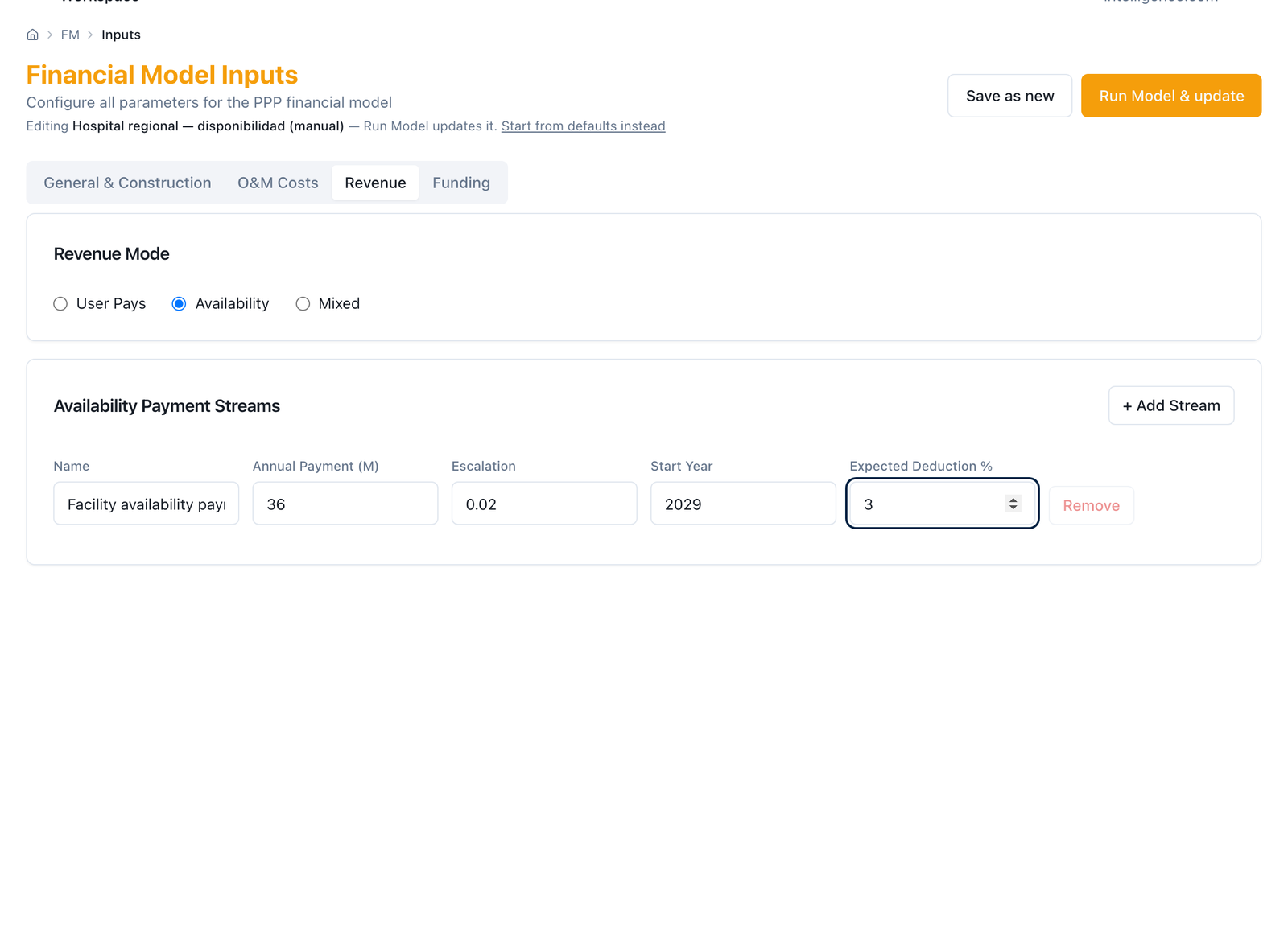
Every figure in the worked example (section 4) and in the screenshots (section 5) is generic: it belongs to the series' hypothetical 300‑bed hospital and to the Coastal Highway of the "Republic of Andolar" demonstration portfolio in FARO, calibrated so that the method can be followed from start to finish. None of it comes from a client or from a real project, and none of it should be used as a reference for the costs, payments or risks of any actual project. The screenshots were taken on the production platform (austral@3116c50e and, for the last two, austral@de6904e5); the version note in §5.1 says what changed between the two. The base against which the floor of a minimum revenue guarantee is compared is, by default, the contract's demand revenue, not its total revenue: under that rule, the Coastal Highway's guarantee is worth 254.8 in the sum over the life of the contract — the figure this manual publishes and the one the platform now reads. The 226.9 that appears in the Financial Model's bankability panel is a second implementation of the same computation — a complete financial model run path by path, against the guarantee engine's revenue simulator — and is declared as such, not as a third, disputed figure. The methodologies cited are credited to their authors; the only product name in the manual is Austral.

Contents

1. What it is for and when it is used
2. International methodological basis
3. The method, step by step
4. Worked example: a hospital under availability, a mixed highway, and the subsidy as an output
5. Implementation on the Austral platform
6. Why not in Excel, for this method
7. References and further reading

1. What it is for and when it is used

A public‑private partnership (PPP) unit has a project that has passed the eligibility screen and whose ex‑ante Value for Money is favourable: a hospital, a highway, a plant. Before writing the tender documents it has to decide something no earlier study decided for it: how the private partner is going to be paid. Who pays — the user, the budget, or both —, per what unit — a month of availability, a vehicle, a bed‑day —, under what conditions — what is deducted if the service fails — and with what adjustment over time — against which index, in what fraction, with what ceiling. And on the other side of the same desk, the Ministry of Finance has the symmetric question: what obligation is born from that decision, of what type and of what size, before approving it.

That is the subject of this manual: the contract clause that turns the risk matrix into money. Everything the matrix says about who bears demand, availability, inflation or the exchange rate is kept or broken in the payment formula: the risk stays with whoever the formula says, not with whoever the matrix says. A matrix that "transfers demand to the private partner" and a mechanism that pays per vehicle with no ceiling have transferred the risk on paper and retained it in the cash box. That is why the payment mechanism is, in the Chilean evidence and in the international evidence, the clause that triggers the most renegotiations when it is designed badly — the guarantee floor that pays in the base case, the indexed tariff with a ceiling and no compensation, the deduction nobody can apply — and the one a well‑made contract renders invisible for thirty years.

The manual reads every mechanism twice over the same figures: as the private partner's revenue, to know whether the contract is financeable; and as an obligation of the State, to know what gets recorded. A mechanism is a formula, a fiscal record and a test in the model, and the manual accepts none of the three without the other two.

1.1 The question it answers — and the ones it does not

The question fits on one line: who pays, per what unit, under what conditions and with what adjustment; and what fiscal commitment is born from it?

Each part does work. Who pays fixes the family of the mechanism — user pays, government pays, mixed — and with it the destination of demand risk. Per what unit fixes the instrument: an availability payment pays for an asset that is ready for use; a usage payment pays for each unit consumed; a subsidy pays for a work built or a service operated. Under what conditions fixes the performance regime: what is deducted, how much, with what rectification period and with what ceiling. With what adjustment fixes escalation and indexation: which index, what fraction of the payment, and what happens when the index reaches where policy will not let it go. And what commitment is born is the fiscal reading of everything above: firm, contingent or State revenue, with its schedule and its present value.

From that follows what the manual does not answer. It does not say whether the project is worth doing: the socio‑economic appraisal decided that earlier. It does not say whether it is worth procuring as a PPP: that is the subject of this series' Value for Money and the Public Sector Comparator manual, which compares the PPP route with traditional public works. It does not say whether the State can afford it: the affordability test lives in that same manual (the maximum payment against the ceiling) and in Fiscal Commitments and Contingent Liabilities (the firm and the expected contingent against the commitment ceiling), and here it is only run as an output check. And it does not allocate the risk the mechanism does not touch: the complete risk matrix — construction, site, change of law, force majeure — is a prior decision the mechanism inherits and makes effective in part.

What the payment mechanism is not

• It is not the risk matrix. The matrix allocates; the mechanism pays. A risk "transferred" in the matrix with no consequence in the formula is not transferred. The manual takes the matrix as given and shows where the formula honours it and where it contradicts it.
• It is not the financing structure. Debt, equity, tranches and covenants are the side that receives the mechanism; the manual uses them to test the formula, not to design them. When the test fails, either the formula changes or the structure changes, and the manual says which.
• It is not rebalancing or tariff regulation. What happens when the mechanism fails — renegotiation, the restoration of equilibrium — and what happens when the tariff is written by a regulator rather than the contract — water, energy, public transport — are frontiers of the method, each treated on one page at the close of §3, not parts of it.

1.2 Where it sits in the cycle

The payment mechanism is decided once per contract and reread three times.

At structuring: the first time. After the ex‑ante Value for Money and before the tender documents, once the project is already eligible and the PPP route is already known to be worthwhile, the PPP unit writes the formula, tests it in the model and records what it creates for the State. This is the moment the formula can still be changed at no cost. The World Bank's PPP Reference Guide places it in contract design, after risk allocation; PFRAM 2.0, in the record the Ministry of Finance makes before approval. Countries that require prior fiscal approval of every contract — Chile, Colombia, Peru — require it at this point, because after signature the mechanism is no longer approved: it is complied with.

At tender: the second time. The bidding variable has to be a parameter of the formula — the lowest availability payment, the lowest subsidy, the lowest tariff, the lowest present value of revenue — and it has to be written with the same symbols as the contract. The formula is reread to fix what is bid and what stays in the tender documents. This is the reading that avoids the most early disputes when it is done, and causes the most when it is not.

With the contract signed: every time something changes. A drop in demand, an inflation shock, a devaluation, a renegotiation request: the same mechanism is reread under the shock to know what the State pays, what it collects and what is left to the partner. The formula does not change; the world changes, and the fiscal record is updated with the original formula and the version of each amendment.

The difference with the Fiscal Commitments and Contingent Liabilities manual lies in frequency and unit: that one runs every year, for the whole portfolio; this one runs once per contract, and its outputs — the firm payment schedule, the guarantee's maximum and expected exposure, expected revenue sharing — are the rows the portfolio register receives. This manual's method ends where that one's begins.

1.3 Who uses it, and for what

Six readers of the same formula, with six different questions.

• The PPP unit, to design and test. It writes the formula with all its parameters, sizes it in the contract's model — the lowest payment, the lowest subsidy, the floor that closes the debt — and tests it with the expected deduction, the demand band and the shocks. It is also the one who has to write down what risk the mechanism left with the State without any clause saying so.
• The sector ministry, to define what is paid for. It writes the service standard the formula remunerates and the indicators the deduction measures; with no output specification there is no availability payment and no deductions (this is the specification criterion of the Eligibility of Projects for PPP manual). An indicator the sector cannot measure is a deduction that is never applied.
• The Ministry of Finance, to approve the type and size of the commitment. It decides whether the State takes on a firm commitment, a contingent one, or none; it sets the rate at which commitments are discounted and the convention under which they are recorded; and it compares the maximum payment with the ceiling. In Austral's partition rule (From Gatekeeper to Orchestrator), the sector writes the service, the PPP unit the formula, and the Ministry of Finance the type and size of the commitment; the sizing, which blends the two halves, goes to whoever holds the financial‑information advantage.
• Bidders and their financiers, to read their cash flow. The formula is their revenue line: debt‑service coverage and equity return come from it with the expected deductions already inside, not from the gross formula. A contract sized gross will be bid net, and the State pays the difference at tender or in renegotiation.
• The comptroller's office, to verify that the bid and the contract are the same formula. The bid was made on one variable; the contract has an annex with the complete formula; if the symbols differ, the contract prevails and the bid is reinterpreted. It is the cheapest check in the cycle, and the one done the least.
• The sector regulator, when the tariff is theirs. In water, energy or public transport, a regulator sets the tariff with its own periodic review; the contract inherits the formula rather than writing it. The method holds in its diagnostic, recording and testing steps; the formula changes hands, and §3 treats it as a frontier.

1.4 The three things the manual delivers per mechanism — and the fourth

For each mechanism, the method produces three things. None is useful without the other two.

1. The formula, complete and with every symbol defined: payment base and unit, schedule and first‑year fraction, escalation and indexation with index and fraction, deduction regime with matrix, rectification period, ladder and ceiling; floor, window, activation condition and band where there is a revenue guarantee; ceiling where the State pays by usage. A formula missing a symbol is not a formula: it is a clause still to be argued over.
2. The fiscal profile: what type of commitment is born — firm, contingent, State revenue or none —, with its nominal schedule and its present value at the policy rate from the base year. Availability payments and subsidies are firm; their conditionality on performance does not make them contingent. A minimum revenue guarantee is a contingent liability with maximum exposure equal to the floor and expected cost by simulation. Revenue sharing is contingent revenue for the State and is recorded separately, never netted. A usage payment is a firm liability of uncertain amount, with a band. The rules are those of the Fiscal Commitments and Contingent Liabilities manual, and step 5 applies them without recomputing them.
3. The bankability test: the minimum debt‑service coverage and the return on equity with the mechanism as it will actually be paid — expected deductions included, the guarantee valued over the demand paths and not over their mean —, and the size of the free parameter that satisfies it: the lowest availability payment, the lowest construction subsidy, the guarantee floor that closes the debt. A mechanism that only closes in the gross base case is not sized.

And the fourth, which almost no contract documents: what risk the mechanism left with the State without anyone writing it down. The political ceiling on an indexed tariff, which turns indexation into an option sold by the State; the high tail of an uncapped usage payment, which is retained demand with no price; the implicit guarantee that the State will not let the concessionaire fail when the floor was set badly. These have no row in the contract; they have a row in this manual's record, with the reason for not valuing them when they are not valued.

There are no numerical thresholds in this section: the required coverage, the policy rate, the subsidy ceiling and the size of the expected deduction are parameters of steps 3 and 4 of the method, and the example in §4 uses them with their stated values.

1.5 Relationship with the Value for Money and Fiscal Commitments manuals

The payment mechanism is the hinge between the two manuals that precede it in the series: it moves Value for Money because it changes who bears demand risk and what leaves the State's cash box; it determines the type of commitment because each instrument is born with its own fiscal record. The table summarises the relationship, instrument by instrument.

A consequence the Value for Money manual anticipated and this one demonstrates: the same hospital that was favourable there under availability at the policy rate changes verdict if it is paid by usage — bed‑day at an equivalent tariff on reference occupancy — because clinical demand risk, which under availability is retained by design and does not enter the comparison, comes to determine the State's outflow. Step 6 walks through it with the Value for Money module; §4 describes it with the example hospital. And the inverse consequence, on the recording side: the same revenue‑guarantee clause, written over the toll or over the partner's total revenue, produces two commitments of different size; §4 shows how much, and step 3 requires stating which.

1.6 What the manual delivers

Three things, in this order.

A self‑contained method. Section 3 develops the eleven steps — from the service frame and unit of account to recording, handover and monitoring — with what goes in, what comes out, how it is computed and what the decision rule is at each one, plus two frontier pages: the regulated tariff and rebalancing. It is written to be run with any tool. Section 2 traces every rule to its source — the PPP Reference Guide, PFRAM 2.0, APMG's certification guide, the British and Australian standardised contracts, and the Chilean contracts of the concessions corpus, cited by article — and says where the sources disagree.

A reproducible example. Section 4 walks the steps through two generic contracts the series' reader already knows: the 300‑bed hospital under an availability payment from the Value for Money manual — where a 3% expected deduction lowers the minimum coverage from 1.208 to 1.145 and requires sizing the net payment — and the mixed Coastal Highway from the Fiscal Commitments manual — with its guarantee floor designed by the official method rather than assumed, revenue sharing valued over the same paths, and the variant in which the State pays the toll —, plus a box in which the construction subsidy is an output of the model rather than an input. Every figure is measured with the platform's engines and a reproducible script prints them; the manual annotates none by hand, and where the engine does not allow something to be measured, it says so.

The tools that run it, and that the client keeps. Section 5 shows how the method runs on the Austral platform: in the Financial Model, where the mechanism is written as the partner's revenue line and tested against the debt — revenue mode, availability‑payment streams, the guarantee and its band, the subsidy sizer, path‑by‑path Monte Carlo —, and in FARO, where the same mechanism is recorded as a State commitment — availability and service payments, the financial liability, the guarantee as maximum and expected contingent, affordability. Section 6 explains why this particular method breaks in a spreadsheet, with seven failures measured on the §4 example. Section 7 gathers the references with their verification status.

A reader who only wants to know whether a mechanism landing on their desk for approval is complete can go straight to the reviewer's checklist at the close of section 3.

2. International methodological basis

Every rule of the §3 method has behind it a guideline a ministry applies, a contract that wrote it, or a paper that explains it. This section says where each one comes from, with section or article, so the reviewer can argue the rule at its source rather than in the manual. Five layers: the three primary sources that give the taxonomy of the mechanism and its place in the cycle (the World Bank's PPP Reference Guide), its fiscal record (PFRAM 2.0) and its checklist (APMG's certification guide); the instrument‑specific guidance that fixed the mechanics — real tolls and shadow tolls on roads, the revenue guarantee as an option, the unitary charge with deductions of the British and Australian standardised contracts, and what the mechanism does not cover and goes to other clauses; country practice, with Chile read in its own contracts; what Austral adds and cites as its own; and table 2.7, which links every step of §3 to its source and to the §5 screen that runs it.

Reading warning. The sources agree on three things: that the payment mechanism is the clause where risk allocation becomes money; that its elements are the same everywhere — who pays, per what unit, under what performance condition, with what indexation and with what guarantee or band; and that a performance deduction is part of the formula, not a penalty. They do not agree on four: whether a usage payment made by the State transfers demand risk or only appears to (the Reference Guide lists it without judgement; APMG calls it "improper transfer" in most cases; the United Kingdom, Spain and Portugal abandoned it); whether payment indexation should be full or partial (HM Treasury requires partial; Chilean practice is full indexation to the UF with one cost‑index exception); whether performance is paid with deductions, fines or bonuses (the British and Australian standards deduct; Chilean contracts fine and reward, and one of them turns performance into term); and whether the revenue guarantee is valued on the mean path or on the distribution (the guidelines say to and almost nobody does). The manual takes a position on each point — a usage payment is a firm liability of uncertain amount and is designed with a ceiling; indexation is declared per stream, with index and fraction; performance is paid with calibrated deductions and a verifier, and the fine is reserved for the breach; the guarantee is valued by path — and presents it as a decision, not as a consensus. The manual's three families and seven instruments are Austral's own formulation of a taxonomy these sources state in different ways; none of them carries this table, and the manual does not attribute it to them.

2.1 The World Bank's PPP Reference Guide, Version 3 (2017)

The PPP Reference Guide, Version 3 (World Bank, ADB and IDB, 2017), module 3 "PPP Cycle", devotes §3.4.2 "Payment Mechanism" (pp. 151–153) to the clause this manual develops, inside §3.4 "Designing PPP Contracts" and after §3.3 "Structuring PPP Projects", where risk allocation is decided. The definition is the one in §1: "the payment mechanism defines how the private partner is remunerated", and "adjustments to payments to reflect performance or risk factors are also important means of creating incentives and allocating risk in the contract". Its basic elements — the list steps 2 and 3 adopt — are four: user charges, collected by the partner directly; government payments, "for services or assets provided", which can be usage‑based ("for example, shadow tolls or output‑based subsidies"), availability‑based ("conditional on the availability of an asset or service to the specified quality") or upfront subsidies against milestones; and bonuses and penalties, "deductions from payments to the private partner, or fines payable by it, when specified outputs or standards are not achieved; or, conversely, bonuses if they are achieved". "A payment mechanism may include some or all of these elements, which must be fully defined in the contract, including the timing and procedure of payment." These are the manual's three families in minimal form: the user pays, the State pays (by usage, by availability or upfront), and the two combine; the deduction is an element of the mechanism, not a punitive clause.

Three subsections give the rules. "Defining user charges": when the concession is paid by tariffs, "the way the tariff is set and adjusted becomes an important risk‑allocation mechanism"; in sectors with monopoly characteristics the tariff "is usually regulated by government, along with service standards", and "the key question for risk allocation is how the tariff will be allowed to change — for example, with inflation or other economic variables, or with changes in different types of cost — and who can trigger a tariff review"; the tariff is controlled "by tariff formulae in the contract, by regulation, or by a combination of both". This is step 3 in its user‑pays branch (base tariff, indexation, periodic review) and the reason for §3's frontier with the regulated tariff: when the formula is not written by the contract, the mechanism has a regulator inside it. "Defining government payments": three considerations — the risk‑allocation implications of each form of payment ("under a usage‑based mechanism demand risk is carried by the private party or shared; an availability‑based mechanism creates an alternative reward not tied to the level of demand"; "an upfront capital subsidy means the private partner bears less risk than if the same subsidy is delivered by availability over the life of the contract", referring to Irwin 2003 on the choice between subsidies); the linkage to output specifications and performance standards, "key to achieving risk allocation in practice"; and the indexation of payment formulae, which "may be fully or partially indexed to certain risk factors, so that government bears or shares the risk". "Defining bonuses and penalties": under government‑paid contracts "bonuses and penalties are typically adjustments to the regular payments"; the Guide stresses "the need to calibrate the payment mechanism — that is, to test the financial impact of penalties under different possible combinations of poor performance —" and refers to the payment‑mechanism chapter of the British standardised contracts (2007 version, chapter 7), "which also describes the calibration of penalties and bonuses on the basis of financial analysis". Step 4's rule — sizing net of the expected deduction — is that calibration written as a model constraint.

Three further points from the Guide that the manual takes as is. §3.3.3 "Translating Risk Allocation into Contract Structure" (p. 144) says that, "besides the allocation of roles, another key element of contract structure is how payments flow", and that the payment mechanism is the way the risk matrix is made enforceable: this is §1's thesis. §3.4.3 "Adjustment Mechanisms" (p. 153) takes out of the mechanism what belongs to rebalancing — force majeure, government action, ius variandi — and refers it to a financial model agreed and maintained through the life of the contract; the manual uses it to draw the boundary of the scope decision. And §3.4.5 "Termination Provisions" brings the third way of fixing the term: besides the fixed contract term and the term as a bidding variable (Mexico), "letting the concession's duration be determined endogenously […] by inviting bids on the basis of the least present value of revenue (LPVR): the concession ends when that value is reached; the more traffic, the sooner it ends", an approach "proposed by Engel, Fischer and Galetovic to manage the risk of fixed‑term concessions and used on roads in Chile and Colombia". This is step 9 and the Chilean counterpoint in §2.5. Lastly, §1.3.3 "The Role of Public Finance in PPPs" (pp. 49–52) sets out the State's financial support — direct loan or subsidy, equity participation, commercial debt guarantee — with the warning that "reducing the capital private parties must contribute reduces risk transfer", and with India's Viability Gap Fund (box 2.9) as an example of an upfront subsidy: the construction subsidy of step 3 and its exit rule in step 4.

What the Guide does not bring: a table instrument → transferred risk → when used. Its elements sit in a list, and the risk reading appears instrument by instrument in the government‑payments subsection; table 2.1 is Austral's own and is presented as such.

Table 2.1 — The Reference Guide's elements and the manual's families and instruments. The correspondence is Austral's own. The Guide does not distinguish families or separate the construction subsidy from the operating subsidy, and treats the revenue guarantee outside the mechanism (§3.3, State support; §1.3.3), where the manual brings it in as a modifier that turns a user‑pays instrument into a mixed one.

2.2 PFRAM 2.0 (IMF–World Bank, 2019): where each mechanism gets written

If the Reference Guide says what each instrument is, the PPP Fiscal Risk Assessment Model 2.0 says where it is written in the State's accounts, and that is why step 5 is its direct heir. Manual M2 verified the sections and this manual does not reread them: §III.C "Government Support to PPPs", §III.D "Accounting and Reporting PPPs" (with the GFSM 2014 and IPSAS 32 control test) and §III.E "Fiscal Risks Matrix". What step 5 takes from them, instrument by instrument: an availability payment is government expenditure in every year and, when the State controls the asset — which happens in almost every government‑paid contract —, the asset and a financial liability equal to the present value of future payments enter its balance sheet from entry into service (§III.D; IPSAS 32, financial‑liability model); this is what FARO's GFS results screen calls the financial liability and computes as the PV of availability plus services (§5). A usage payment made by the State is the same expenditure with an uncertain amount: PFRAM models it as government‑paid services with a quantity and a price, and the manual classifies it as a firm liability of uncertain amount, not as contingent, because the obligation exists in every state of the world and only its size depends on demand. User tariffs are the partner's revenue and do not touch the State's accounts unless the contract assigns them to it (tariff‑based service payment, §III.C, financing type "Government Payment (Tariff)") or the State collects royalties and other payments, which are revenue. A construction subsidy is a capital transfer in the disbursement years; an operating subsidy, current expenditure. A minimum revenue guarantee and a debt guarantee are explicit contingent liabilities with maximum exposure and expected cost (§III.C: guaranteed price and volume that "together determine the minimum guaranteed revenue amount"; percentage of debt guaranteed), and the risk matrix (§III.E) lists demand, financial equilibrium and renegotiation as categories where the mechanism is reread. Revenue sharing has no row of its own in PFRAM: the manual records it as contingent revenue for the State, separate and never netted against the guarantee's expected cost, with M2's rule (one obligation, one row; mutually exclusive by the larger).

Two positions the manual takes beyond PFRAM, stated as such. First: performance conditionality does not make a payment contingent — an availability payment that can be reduced by deductions remains firm, with the expected deduction as an estimate of its size (M2, step 2) —; PFRAM does not contradict this, but it does not state it either, and the confusion is frequent in national registers. Second: a usage payment is recorded with its band (P5–P95 of demand) and not only its mean, because a firm liability of uncertain amount with no band is an underestimated firm liability; PFRAM delivers revenue sensitivity and the manual uses it to write the band.

2.3 APMG (2016): the formula's checklist

The APMG Public‑Private Partnership (PPP) Certification Guide (APMG International, with the ADB, the EBRD, the IDB, the IsDB and the World Bank, 2016) brings, in chapter 5 "Structuring and Drafting the Tender and Contract", the most complete section that exists on how to write the formula: section 4 "Financial Structuring (from the Public Perspective): Defining the Financial Structure and Payment Mechanism" (pp. 28–72). Its order is that of steps 2 and 3: §4.1 the term (with the question of the optimal term); §4.2 pure co‑financing — the construction subsidy, with the Chilean example: "the financial scheme of PPP hospitals in Chile is based on two payment streams: an operating payment (subject to deductions and adjustments for quality and availability) and a fixed construction payment (which is in fact a long‑term deferred subsidy)"—; §4.3 public loans; §4.4 "Filling the Viability Gap of a User‑Pays Project"; §4.5 equity participation; §4.6 other ways to increase feasibility, where the minimum revenue guarantee appears as a contractual guarantee ("government payments to the partner if revenue falls below certain levels, for example in South Korea, or under more sophisticated schemes, such as the Chilean road model, in which the term is extended until revenue reaches an agreed PV"); §4.7 the categories of revenue regime — user pays, government pays, and the four reasons why an economic‑infrastructure project ends up government‑paid, among them "it may be decided that no charge is made (a toll‑free highway): it is a public‑finance decision whether the project is financed with charges to specific users or with tax revenue"; and the case where there are tariffs but the partner receives only government payments, with the State retaining the tariff revenue "to retain the risk and reward of collection" (I‑595 in Florida, Portugal's former SCUTs) —; §4.8 the structuring of user‑pays projects (toll levels and structure, review and indexation — "in some countries, for example Spain, a correction factor is included to incentivise efficiency: tariffs indexed to 0.85 × CPI" —, term, traffic guarantees); §4.9 volume‑linked mechanisms; and §4.10 availability payments, in eleven subsections that are step 3's checklist: definition of availability and failure categories (4.10.1), composition of the unitary charge and time apportionment (4.10.2), adjustment factors or deductions (4.10.3), weighting by time band (4.10.4), rectification periods (4.10.5), escalation ladder for repeat failures (4.10.6), maintenance and other exceptions (4.10.7), payment indexation (4.10.8), first payment and early termination (4.10.9), other payments and adjustments (4.10.10), and frequency and computation process (4.10.11).

Four rules of step 3 come from this guide, almost verbatim. On the usage payment (§4.9): "volume‑risk structures should only be considered where there is a clear alignment of interests (the public side wants more demand) and where traffic risk is considered reasonably assessable and manageable by the private partner"; table 5.2, "improper and proper transfer of volume risk", places on the improper side the treatment plant paid per m³ with no take‑or‑pay, the hospital paid per occupant and the toll‑free highway paid per vehicle — "if there are many more users than expected, government payments will be much higher than budgeted" —; and on bands: "regardless of whether there is a banding system, there must be a maximum traffic level above which government does not pay", with a small shadow tariff above that maximum as an approximation of the marginal cost of operation. Step 3's rule — with no ceiling, the State retains the whole high tail — is this one. On indexation: a fixed factor (2% a year) "is of doubtful rationality, because government will end up paying the price of transferring inflation risk"; and in availability payments (§4.10.8) "many projects opt for a composite formula in which only a proportion of the unitary charge is adjusted for inflation", because "debt service is generally not linked to inflation" and indexed costs "usually represent less than 50% of total disbursements". On deductions (§4.10.3): they must be "proportionate to the severity of the criterion breached and of the failure", weighted by area, duration, time band and persistence, and "in some social‑infrastructure projects a deduction may be greater than the value of the payment theoretically obtainable during the unavailability period" (150–200% in the British guide), although "the actual deduction is always capped at 100%". On rectification (§4.10.5): "not every failure should have a rectification period" (food in a prison, energy in a hospital), and "rectification periods should not disincentivise preventive maintenance". And a warning the manual carries into step 7: "the payment mechanism must be applied in practice" — HM Treasury says the same (§2.4) — because a deduction the authority does not collect so as not to damage the relationship with the contractor is a deduction that does not exist.

The guide also says where the mechanism is put out to tender (chapter 5, §8.2): price‑based evaluation "only" admits variables such as the availability payment, the tariff or the subsidy; "an exception in more sophisticated approaches (for example, the Chilean one for real‑toll highways) is to bid and evaluate on the PV of revenue: not only a price‑evaluation mechanism but also one of risk sharing, because the term becomes variable to meet the bid PV". This is half of step 9; the other half — one variable, one formula — is Austral's own.

2.4 The instrument‑specific guidelines

Roads: real tolls, shadow tolls and availability. The Toolkit for Public‑Private Partnerships in Roads and Highways (World Bank and PPIAF, 2009; six modules, with module 2 "Key Components" on risk, financing and public accounting and module 4 "Laws and Contracts" on the contract) is the sector guidance that orders the three ways of paying for a road and the risk each one leaves with the State; its payment‑mechanisms note sits in module 6's bibliography. The shadow‑toll mechanics the manual cites come from its British origin: in the United Kingdom's first DBFO (Design, Build, Finance and Operate) contracts, reviewed by the National Audit Office in 1998, bidders proposed up to four shadow tariffs for four traffic bands, with the top band's tariff fixed at zero, "limiting government's financial exposure to toll payments even if traffic grew". This is the source of step 3's "tariff by volume band, declining, with a ceiling", and also of the judgement the manual shares with APMG: the instrument transferred demand the private partner did not control, and the United Kingdom, Spain and Portugal replaced it with availability (§2.5).

Irwin (2007), Government Guarantees. The revenue guarantee is an option the State sells: its cost is expected and its exposure is maximum, never a fixed budget line; the book's "allocate, value and record" framework is that of M1 and M2, and the manual does not reread it. From the same author comes step 2's rule that each instrument is chosen with its record in view: the guarantee, Irwin writes, is often preferred because it does not appear in the budget, and the remedy is to value it before granting it. Step 5 is that remedy applied to the whole mechanism.

The British standardised contracts. The Standardisation of PFI Contracts, Version 4 (HM Treasury, March 2007, SoPC4) devotes its chapter 7 to the payment mechanism — the chapter the Reference Guide cites for calibration —, and its successor, the Standardisation of PF2 Contracts (December 2012), rewrites it as chapter 19 "Price and Payment, Availability and Performance Mechanism" with chapter 20 "Payment Mechanism and Monitoring". The manual takes from the 2012 version (as read) the deduction rules, which SoPC4 already contained. The mechanism's features (§19.2.1): "no payment before service commencement; a single unitary charge for the service, not made up of separate availability and performance elements; the level of payment linked to the level of service; the charge never paid in advance; the mechanism adjusts for poor performance and deductions reflect the severity of the failure — no service, no payment, but a minor failure causes a minor deduction, except for persistent failure, where escalation mechanisms may increase the deduction —; a balance between the mechanism's variables — the initial weighting of deductions, response and rectification periods, the ladder for repeated failures —; the charge based on outputs, not inputs; and payment that is fully auditable". It is not appropriate to "sculpt" the charge with an irregular profile for affordability reasons (§19.2.2), and "the mechanism must be applied in practice: there have been occasions where authorities have been reluctant to impose deductions for fear of damaging the relationship with the contractor" (§19.2.3). Usage‑based systems (§19.4) are admitted "where the contractor's performance can influence the level of use" and are distinguished from third‑party income with gain‑sharing. Availability (§19.5) requires a definition that is "objective, measurable, reasonable, achievable and material", with the case of space "unavailable but used". Performance (§19.6) is fixed by outputs and measured with a points regime. Calibration (§19.7) — "assigning numbers to the parts of the mechanism" — "is central to value for money", "should avoid high levels of deduction when overall performance is good", and must be completed "before appointing the preferred bidder, with a commitment not to ask for recalibration afterwards". And indexation (§19.11): "it is not usual for the whole unitary charge to be indexed, and such over‑indexation should not be used to artificially reduce the initial charge"; value for money "is achieved by indexing the proportion of the charge that corresponds to the contractor's non‑fixed costs, with a general index such as the RPI", and the authority fixes the index and leaves the indexed fraction to the bidder (§19.11.3). The chapter closes with the no double remedy rule (§19.12): the deduction and the fine do not accumulate over the same failure, which is the manual's distinction between deduction and breach.

Australia. Infrastructure Australia's National PPP Guidelines place the mechanics in two volumes of commercial principles: volume 3, Commercial Principles for Social Infrastructure (December 2008), for availability‑paid contracts — with the abatement regime for payment on unavailability and performance —, and volume 7, Commercial Principles for Economic Infrastructure (February 2011), for contracts with third‑party revenue and demand risk on the private partner. The distinction between volumes is the manual's distinction between families, and the term "abatement" is what Australian practice uses where British practice says deduction.

What the mechanism does not cover. The World Bank's Guidance on PPP Contractual Provisions, 2019 Edition orders the clauses that surround the mechanism and that the manual does not develop: force majeure, authority adverse events (MAGA), change of law, step‑in rights, termination events and termination payments, asset handback and dispute resolution. Step 8 refers to them with the rule that the payment formula must say what it does not cover and which clause it goes to. And the World Bank's compendium on the fiscal implications of PPPs (2022, by the manual's own author) documents what happened to demand guarantees and rebalancing under the pandemic: this is §1's evidence that a badly sized mechanism is the clause that triggers the most renegotiations.

2.5 Country practice

Table 2.5 — How countries pay. Dominant instrument in the programme, the State's payment unit where there is one, indexation, how performance is treated, revenue guarantee and bidding variable. Always clauses, never performance figures.

Chile is the country that combines the most instruments in a single programme, and the manual reads it in the contracts of the concessions corpus, with the contract, the document and the article. Four observations no international guideline brings.

First: the Chilean availability payment is called a subsidy and is bid as an instalment. In the Maipú and La Florida Hospital concession, the tender documents separate the Subsidio Fijo a la Construcción (Fixed Construction Subsidy, art. 1.12.3.1: the Ministry of Health pays for each hospital eight annual instalments from the payment authorisation, with a fraction per hospital), the Subsidio Fijo a la Operación (Fixed Operating Subsidy, art. 1.12.3.2: advance semi‑annual instalments, with the first and last at half instalment) and the Pagos Variables a la Operación (Variable Operating Payments, art. 1.12.3.3), where each hospital's Variable Operating Subsidy is SVO = PVC × max(NCR − NC, 0) + PA + CP + RS: a payment for each additional bed‑day of 0.5 UF over the reference occupancy of the contract, plus payments for new investment, compensation for bed over‑demand (art. 1.12.4) and the Service Result. The two bidding factors are the SFO's semi‑annual instalment and the SFC's annual instalment (arts. 3.1.1 and 3.1.2), each with a maximum set in the tender documents (art. 3.2), and the bid is evaluated by a score combining the present value of both (art. 3.3). The SFO is partially indexed to a labour‑cost index: "only if variations occur in the Monthly Minimum Wage set by law will 20% of the SFO be adjusted according to the variation that this Minimum Wage has shown relative to the one in force when bids were submitted" — SFO_j = SFO × (0.8 + 0.2 × Wmin_j / Wmin_0) — (art. 1.12.11), on a base already denominated in UF. This is exactly APMG's and HM Treasury's "composite formula", with a cost index instead of the CPI, and the manual uses it as an example of indexation by stream with a declared index and fraction (step 3).

Second: performance in Chilean hospitals is not deducted; it is fined and rewarded. The service‑level mechanism is not in the "Document No. 12" the original tender documents cited, but in article 1.10.17, "Mecanismo de determinación de niveles de servicios" (Service‑Level Determination Mechanism), added by Clarifying Circular No. 1 to the tender documents, which also corrected the definition of the Service Result. Each service has a semi‑annual Partial Service Level, NSP = 100 − Σ N_j × P_j (breaches by points of relevance), and each hospital an Overall Service Level weighted by relevance factors (from 0.005 for the cafeteria to 0.160 for food service). A deficient NSP (below 92 points) in any service triggers the fines of table 4, art. 1.8.5.1; a good or excellent NSG (94 or 97 points), with every service above threshold and no breaches of the sentinel indicators (art. 1.10.18), earns a fixed semi‑annual incentive in UF paid once a year inside the variable subsidy as the Service Result. The text says so itself: the mechanism "is intended to generate incentives for adequate service provision, and in no way constitutes a guaranteed incentive". In other words: the SFO instalment does not fall with performance; the failure is sanctioned as a breach and excellence is rewarded as a bonus. APMG's guide describes the operating payment of Chilean hospitals as "subject to deductions and adjustments for quality and availability"; the contract as read does not deduct. The manual flags it because the difference matters at step 5: a fines‑and‑bonus regime does not change the SFO's firm nature, but it leaves performance outside the formula, and step 4's calibration has nothing to act on.

Third: a usage payment made by the State exists in Chile, with an implicit ceiling and no deductions. In the Group 1 Prison Programme, the Ministry of Justice pays semi‑annually, for each of the three facilities, a third of the SFC instalment (twenty‑one calendar semesters, the first and last fractional), a third of the SFO instalment, and "the result of multiplying the Average Number of Inmates (NPI) of the previous semester by the Variable Payment Indicator (IPV)" bid (art. 1.12.3, "Payments from the Ministry of Justice to the Concessionaire", whose general expression sums the three components per facility and adds the early‑termination payment). These are the three bidding factors (art. 3.1: SFO semi‑annual instalment, IPV per inmate‑semester and SFC semi‑annual instalment, each with a maximum in art. 3.2). The usage payment has an overcrowding correction that acts as a declining ceiling: if the NPI exceeds 120% of design capacity, the IPV applies in full up to that 120% and, for the excess, is adjusted by a factor (art. 1.12.9) — the British shadow toll's declining band, written for inmates. And there are no deductions: performance is sanctioned with the fines of art. 1.8.5.1. For step 3 this is the example of a usage payment with a unit, a tariff by band and a ceiling; for step 5, a firm liability of uncertain amount the tender documents do not cap from above except by that curvature.

Fourth: the revenue guarantee and revenue sharing were written as the bidder's option, with activation and a band. On the Route 5, Santiago–Los Vilos section, art. 1.11, "Distribución de riesgos entre la Sociedad Concesionaria y el Estado" (Risk distribution between the Concessionaire and the State), offers an optional mechanism: a bidder who accepts it chooses, year by year, a Minimum Guaranteed Revenue within the lower and upper band of table 1.2, with a ceiling on the updated sum; in exchange, it "must share 50% of its revenue in the event that profitability exceeds 15%". The guarantee activates only if the year's revenue is below the guaranteed minimum and above 50% of the potential revenue computed at the reference tariff: step 3's "the guarantee does not cover an operator that does not operate" is this clause. Revenue sharing applies "for the following month in which" the updated value of monthly revenue at a real annual rate of 15% exceeds an amount in UF fixed in the tender documents, and from then on the concessionaire pays the MOP 50% of its revenue. The Puente Industrial (Industrial Bridge) repeats the design with a payment from the concessionaire to access the guarantee, and a waiver (art. 1.12.2.1.2; the mechanism, in art. 1.12.7.1). And term‑based revenue distribution appears when the mechanism fails: Supplementary Agreement No. 3 of Route 5 Chillán–Collipulli (2004) modifies "the degree of risk commitment the Concessionaire Company assumes […] regarding variations in vehicle flow, establishing a variable‑term concession system" (clause 4.2), in exchange for a payment from the concessionaire on access (clause 5.1) and with a single "Revenue Distribution Mechanism Account" updated at a fixed monthly real rate (clause 5.3): the MRG and revenue sharing rewritten as an account that decides when the contract ends.

And the bidding variable that absorbs demand risk through the term. Route 68 (Santiago–Valparaíso–Viña del Mar Road Link) fixed, by clarifying circular, a single bidding factor, the Total Concession Revenue (ITC) in present value (art. 3.1.1 after the amendment; arts. 3.1.3 and 3.2 of the original text, with the base tariff and maximum term set in the tender documents), and the concession "shall be extinguished in month m when" the present value of monthly revenue, discounted at the risk‑free rate plus a 5% real premium, reaches the bid ITC (art. 1.5.6), with extinction upon reaching the ITC (art. 1.9.2) or, if not reached within 300 months, by maximum term "with no right to indemnity or any compensation for the difference" (art. 1.9.3). The tender documents invoke the legal basis for the factor "used exceptionally" (Concessions Law, art. 7, letter l) and give the reason: to allow a future joint re‑tender with a new corridor. The Route 78 re‑tender (Santiago–San Antonio Highway, tender documents in process in the corpus, not yet registered by the Comptroller) takes the design to its mature form: the ITC as the sole factor (arts. 3.1–3.4, with a maximum in UF), extinction when the VPI reaches the ITC (art. 1.7.6), the VPI computed at a fixed 2% rate plus a 2% real premium (art. 1.7.6.1) and — this is new — a quarterly Service Delivered Index (art. 2.4.6.5) that credits the concessionaire an Operational Performance Incentive proportional to the excess over 0.970 and charges it an Insufficient Operational Performance Cost by bands when it falls below; both are recorded in an Operational Performance Fund whose negative balance is deducted from the VPI. Performance does not reduce a payment: it lengthens the concession. This is the only version of a performance deduction in the corpus that enters the formula, and it enters through the term. Step 7 cites it as proof that a deduction can be written in any unit — money, points or months — provided it has a verifier.

And the subsidy as an output, written into a set of tender documents. The Puente Industrial was tendered in two mutually exclusive tracks (art. 3.2): track A, with the ITC as the variable and zero subsidy; track B, with a Subsidy Factor S between 0 and 1 that multiplies ten annual construction‑subsidy instalments fixed in the tender documents (art. 1.12.1.1, table 6) and the ITC fixed at its maximum. "The concession shall be awarded to the bidder who bids on track A […]; in the event that no bidder submits a bid on track A, the concession shall be awarded to the bidder who bids on track B" with the lowest S (art. 3.4). The market is asked first whether the project closes with no subsidy; only if nobody answers is the subsidy sized, and it is sized by competition. This is "minimise before subsidising" (§2.6) written into a set of tender documents called in late 2012.

Urban tariffs. The Norte–Sur System (Autopista Central) defines three tariffs per kilometre — off‑peak, peak and saturation — triggered by the road's operating speed (art. 1.14.1), with maximum factors by vehicle type (art. 1.14.2), and adjusts them every 1 January by T_t = T_{t−1} × (1 + CPI) × (1 + RR), where RR is "the maximum real annual tariff adjustment the Concessionaire Company may apply", 3.5% from the second year on; if the CPI accumulated since the last adjustment exceeds 15% in any month, the tariff is adjusted early, and every two years the concessionaire may request a review of the adjustment system, "which the MOP may accept or reject with the endorsement of the Ministry of Finance" (art. 1.14.7). Full indexation to the CPI plus a cumulative real rate, with no contractual ceiling: the case The Indexation Ceiling (§2.6) uses to ask who pays when the political ceiling arrives before the formula does.

United Kingdom. The PFI/PF2 unitary charge with deductions for unavailability and performance is the standard §2.4 describes, and the National Audit Office has documented its full cycle (the 1998 DBFOs; PFI and PF2, 2018). The shadow toll of the 1990s DBFOs — up to four traffic bands, the top one at zero tariff — was the first version of the usage payment with a ceiling; it was abandoned because it paid the private partner for traffic it did not control, and the next generation of roads moved to availability with congestion measures (APMG, §4.9). PF2 was abandoned in 2018; the manual cites its rules as method.

Australia. Abatement of the availability payment in social infrastructure (volume 3) and demand risk on the private partner on roads (volume 7), with the warning Australian practice itself put in writing: the traffic failures of the urban real‑toll tunnels (Sydney, Brisbane) are the empirical argument of Bain (2009) and of APMG's table 5.2 against transferring demand nobody controls, and the reason for step 1.

Colombia. Law 1508 of 2012 defines a PPP as a contract "that involves the retention and transfer of risks between the parties and payment mechanisms related to the availability and level of service of the infrastructure and/or service" (art. 1), and its article 5, "Derecho a retribuciones" (Right to Payment), makes conditionality a norm: "the right to collect resources from the economic exploitation of the project, to receive disbursements of public resources or to any other payment […] shall be conditional on the availability of the infrastructure, on compliance with service levels and quality standards in the project's different functional units or stages"; later paragraphs allow payment by functional units and by stages, always conditional. This is the only country in the table where performance conditionality is a legal requirement of every payment, and the record of the firm liability is the future budget appropriations (art. 26). The 4G programme added guaranteed revenue through a collection shortfall mechanism on toll highways.

Peru. Co‑financed PPPs pay the investment with a Retribución por Inversión (RPI, Investment Payment, or RPI‑CAO against progress certificates, as on Metro de Lima Line 2) and operation with a Retribución por Mantenimiento y Operación (RPMO, Maintenance and Operation Payment); the first generation of roads used the PAO and the PAMO with the CRPAO — a negotiable certificate of annual works‑payment recognition — as a tradeable title. The progress certificate as a payment title is the Peruvian form of step 3's construction subsidy against milestones, with a consequence step 5 records: once issued, the certificate is an unconditional firm liability, and performance conditionality falls only on the RPMO.

Mexico. Proyectos para Prestación de Servicios (PPS, public‑service‑provision projects) — an agreement of the Secretaría de Hacienda and the Secretaría de la Función Pública, published in the Diario Oficial on 9 April 2004, updating the March 2003 rules — are the availability payment with deductions budgeted as current expenditure, the clearest form of step 5's rule that an availability payment is the year's expenditure; the 2012 Public‑Private Partnerships Law inherited the scheme.

India. The hybrid annuity model (HAM), approved in January 2016 for national highways, pays 40% of construction cost during construction against milestones and 60% in semi‑annual annuities with interest through the concession; the PPP financial‑support scheme (VGF) subsidises up to 20% of cost from the central fund and up to another 20% from the sponsoring entity. This is the construction subsidy combined with a firm liability, the form the manual calls mixed government‑pays and that §4(c) runs through the VGF solver.

Spain and Portugal. The Spanish regional shadow toll and Portugal's seven SCUT concessions — "sem custos para o utilizador" (no cost to the user), some 930 km built between 1998 and 2002 with the imported British model — are the case study of an instrument that appears to transfer demand and does not: Portugal introduced real tolls in two waves (late 2010 and late 2011), renegotiated the contracts to availability payments with the State retaining the tariff revenue (APMG, §4.7), and its Tribunal de Contas (Court of Auditors) audited that renegotiation [to be verified: the report's conclusions]; since the early 2010s, every Spanish project has used availability (APMG, §4.9).

Where they diverge, on four axes. Whether the deduction is a discount, a fine or a bonus: discount off the charge (United Kingdom, Australia, Mexico, Peru on the RPMO; Colombia by law), fine for breach plus bonus (Chilean hospitals), term (Route 78 re‑tender). Whether indexation is full or partial: partial by rule (United Kingdom; APMG) or full to an indexed unit with a cost exception (Chile, UF and 20% to the minimum wage) or full to the CPI plus a real rate (Chilean urban highways). Whether the revenue guarantee carries a band: optional with activation and revenue sharing (Chile, Los Vilos and Puente Industrial), by term (Chile, ITC and MDI), by collection shortfall (Colombia), no guarantee (United Kingdom, Australia). What variable is bid: the payment (unitary charge, RPI + RPMO, annuity), the subsidy (SFC/SFO, factor S), the PV of revenue (ITC), or two mutually exclusive tracks. The manual takes a side at step 3 and step 9: deduction inside the formula, indexation by stream with a declared fraction, guarantee with activation and a band, and one bidding variable with the same symbols as the contract.

2.6 What Austral adds and cites as its own

Six rules in §3 are not in any of the guidelines above in the form the manual uses them, and are attributed to Austral.

The mechanism is where retention is decided (step 1, step 2). The maxim "allocate each risk to the party best able to manage it" — repeated by the Reference Guide, APMG and every national guideline — "is correct, is intuitive, and is almost never quantified" (Austral, The Optimal Risk‑Retention Frontier, §1). The paper separates managing from bearing, shows they come apart for macro risks — aggregate demand, the exchange rate — and adds "at a reasonable cost" (§4): there is a ceiling beyond which the private partner will not take the risk at any price. For the payment mechanism the consequence is one of design: transferring demand risk is worth what the private partner manages minus what it charges to bear it, M − P, and no more. A usage payment with no ceiling is retention with no price (the State keeps the high tail and does not write it down); a minimum revenue guarantee is retention with a price (the State keeps the low tail and records it). Step 1 asks whether the private partner controls, diversifies and can price demand before choosing a family, because the frontier says transfer creates value only when the answer is yes.

The subsidy is an output of the model, not an input (step 3, step 4, §4c box). "The language of 'closing the gap' presents it as an input — a fixed amount, sitting in the project, that a subsidy covers. It is none of that. The gap is an output: the residual left over after choosing the risk allocation and the financing structure" (Austral, The Viability Gap Is an Output, §3). The sequence — minimising the gap, sizing the residual as "the smallest subsidy that satisfies bankability, value for money and affordability at once" (§4), recognising it as a commitment (§7) — is step 4 in its subsidy branch, and the platform's VGF solver is its implementation. The Puente Industrial's two‑track tender (§2.5) is the same rule written into a set of tender documents: the market answers first whether there is a gap, and only afterwards how much it is worth.

The guarantee is valued over the distribution, never over the mean path (step 4, step 5). This is manual M2's valuation rule (§2.6 of that manual), which step 4 takes one step further: it is not enough to simulate the guarantee separately and add its expected cost to deterministic revenue; path Monte Carlo delivers the complete model to every state of the world, and in each one the partner receives max(R, MRG) − x·max(R − UB, 0) and the State pays and collects out of that same draw. The author's own precedent: the official Chilean methodology for sizing the MRG (Duarte Arancibia, 2015, §6.1, equations 11–17): the present value of risk‑free revenue equals the present value of maximum debt, with a profile MRG_t = MRG_1·(1 + g)^(t−1) and a symmetric upper band UB = 2·E − MRG; the platform implements it and step 3 adopts it. The manual cites Austral's note on the third‑party guarantee decision (Foundations for Deciding When to Use a Third‑Party Guarantee) only for what it says — when to compare the sovereign guarantee with a third‑party one (§2.2–§2.6) —, not for path valuation, which that paper declares outside its scope (§11).

Indexation is a sold option, with a ceiling (step 3, user pays). "Embedded in every indexed tariff is an undeclared assumption: that government will let the tariff rise by the full index, every year, for the life of the contract. That assumption is a political variable, and it fails in a predictable way" (Austral, The Indexation Ceiling, §1.1). When the index passes the ceiling, government "caps the increase and finds another way to keep the operator whole" (§1.2); what the State has sold is a call option on the index with a strike price at the ceiling, payment_t = revenue_t × max(0, g_t − C) / (1 + g_t) (§3.1). Step 3 requires, for every adjusted tariff, a ceiling‑compensation clause, and step 5 records the option when the clause does not exist. The Silent FX Liability is the zero‑ceiling case: FX indexation "is the special case of an indexation clause with a zero affordability ceiling" (Indexation Ceiling, §3.2), and that is why step 3 admits it only for the fraction of costs in foreign currency. The Norte–Sur System's formula — CPI plus a cumulative 3.5% real rate, with no contractual ceiling and a biennial review subject to the Ministry of Finance's endorsement — is the Chilean example the manual uses to illustrate the question.

The mechanisms that invite renegotiation (step 3, step 8). The Renegotiation Triangle prices the three exits of a renegotiation — accept, counter‑offer, terminate — (§2) and measures in the Chilean panel that renegotiation is "endemic and right‑skewed" (§4). What the manual takes from it is the list of causes born in the mechanism: a guarantee floor set on the base‑case path, which pays in the base case and is no longer a guarantee; a ceilinged tariff with no compensation clause; a deduction with no rectification period and no verifier, which is disputed instead of applied; and a bid formula different from the contract's. Step 8 turns these into a clause checklist. And Three PPPs — A Walkthrough runs three payment structures end to end on the platform; the manual cites it for the walkthrough, with the warning that its figures are illustrative and not those of the §4 example.

Where it is recognised and who decides (step 5, §1.3). The Recognition Rule orders the four lenses under which an availability payment does or does not enter the State's balance sheet (§2–§4) and shows where the line is fought over (§6); step 5 adopts its rule that the firm/contingent classification is written with the declared lens. The PPP Budget Nobody Publishes gives the envelope against which step 6 tests the maximum payment, and Stress‑Testing PPP Portfolios the reason the mechanism's stress must be read at portfolio level (§2: a common stress does not diversify). From Gatekeeper to Orchestrator (§2.4, the partition rule) orders who decides what in the mechanism: the sector writes the service and its indicators, the PPP unit the formula, the Ministry of Finance the type and size of the commitment and the rate; the step that blends the two halves — step 4's sizing — goes to whoever holds the financial‑information advantage.

A contradiction the manual does not soften: the Reference Guide and APMG describe the government‑paid usage payment as an instrument "that shares" demand risk; read through the retention frontier, with no ceiling it shares nothing: it retains the high tail with no price and transfers the low tail to whoever does not control it. The manual calls it a firm liability of uncertain amount and designs it with a ceiling, and that is a position, not a consensus.

2.7 Correspondence table: §3 step → source → §5 screen

3. The method, step by step

This section is the complete method, written so that someone with their own financial model and fiscal register can apply it without the platform: each step says what goes in, what comes out, how it is decided and what the rule is. The sourcing of each rule is in §2 and is not repeated; the Chilean counterpoints that illustrate it are in §2.5 and are cross‑referenced; the figures that illustrate the steps are those of §4 and are explained there; the formulas for each instrument, with all their symbols, are in annex 3.A at the end of the section. The method has eleven steps and two frontier pages: from the frame (step 0) to recording and monitoring (step 10), and after that the tariff a regulator sets (3.12) and rebalancing (3.13), which the manual delimits and does not teach.

Three warnings before starting. The first is the manual's thesis: a payment mechanism is a formula, a fiscal record and a test in the model, and the method accepts none of the three without the other two — a formula with no record is an obligation nobody wrote down; a record with no test is a commitment nobody knows whether the contract can pay; a test with no formula is another contract's model. The second: the method applies to a project that has already passed the eligibility gate (M3) and whose Value for Money has already been measured with an assumed mechanism (M1); what it does is replace that assumption with a clause and measure again. The third: each step produces something the next step consumes and the reviewer can ask for; the list in 3.11 says what.

Step 0 — Frame: the service, the unit of account and today's payer

In. The output‑based service specification (M3, criterion 2: what the contract requires to be available or delivered, not the inputs it is made with); the contract's horizon (works plus operation) and the base year; the financing currency and the local currency, with the inflation of each; who pays today for the equivalent service — users, the budget, nobody — and at what tariff; and the policy rate at which the Ministry of Finance discounts commitments.

Out. The convention that governs the formula, in one line at the top of the record sheet: "service X specified by outputs; unit of account Y; currency Z of base year, nominal, N‑year horizon from start year; today's payer: W". The unit of account is this step's decision: availability by functional area (hospital, prison, building), by lane‑kilometre (road), by vehicle or passenger (usage), by bed‑day or inmate‑semester, by m³ or MW (services). Everything that follows is written in that unit.

How it is decided. There is no computation, there are three definitions. (i) The unit of account is that of the output the contract buys: if the State buys an available hospital, the unit is availability weighted by area and time band; if it buys care, it is the bed‑day; if the user buys passage, it is the vehicle. A unit the verifier cannot count (step 7) is no use as a unit of account. (ii) The horizon and the base year are those of the project model (M1, step 0): the mechanism is tested in the same model, with the same convention, and the commitment's present value is computed from the base year, with the base year undiscounted (the Fiscal Commitments manual's convention). (iii) The payment currency is decided here, not in step 3: a State payment in the financing currency shifts the whole exchange‑rate risk onto the State; in local currency with partial FX indexation, only the indexed fraction (step 3, Silent FX Liability).

Decision rule. A service that cannot be specified by outputs admits neither an availability payment nor deductions (M3, criterion 6): either the specification is resolved or the service is paid by inputs, in which case it is not a PPP. And today's payer is declared even if it is "nobody": a service that is not charged for today and will be charged for tomorrow (a new toll) carries an acceptance risk step 1 must read before choosing a family.

Where teams go wrong. Taking the financial model's unit — "annual revenue" — as the unit of account instead of the contract's: step 3's formula needs a unit measurable on the ground, not a spreadsheet line. And fixing the payment currency for the financier's convenience ("in dollars, because the debt is in dollars") without writing it down as a risk‑allocation decision: §4 shows the hospital paying in nominal dollars with fixed 2% escalation — the demo package's choice — and box 4.8a shows the Chilean case paying in UF with 20% indexed to the minimum wage; both are decisions, not details.

Step 1 — Diagnosing demand risk and ability to pay

In. The demand forecast with its band (P10–P90, or a declared annual volatility), not only its mean; price elasticity; the user's ability and willingness to pay and the existence of free alternatives; the sector's documented optimism bias (toll traffic forecasts overestimate by 20–30% on average: Bain 2009; Flyvbjerg et al. 2005); and Austral's three retention questions (The Optimal Risk‑Retention Frontier): does the private partner control demand? can it diversify it? can it price it at a reasonable cost?

Out. The diagnosis in four boxes, with the band in view:

And with the diagnosis, the risk measure the rest of the method will use: the annual volatility of demand revenue (15% in the series' convention when there is no own estimate, from the Fiscal Commitments manual) and the P10–P90 band of the first and last year.

How it is decided. The three retention questions are answered about demand, not about the project. Controlling is being able to move it with what the contract lets the partner do (quality, collection, marketing): an inter‑urban toll is barely controlled; a hospital bed, not at all; a parking lot, quite a lot. Diversifying is being able to offset it with other demands of the same partner: an operator with one road does not diversify; with twenty, it does. Pricing it means a market exists — financiers, insurers — that charges to bear it at a cost the State is willing to pay in the tariff or the payment. Three "no"s is box B; three "yes"es is box A; "chargeable but neither controllable nor diversifiable" is box C. The band discounts the bias before choosing: if the sponsor's forecast carries no band, the sector's is imposed on it, and if it carries no optimism correction, step 4's path Monte Carlo applies it as a declared parameter (§5).

Decision rule. Demand the private partner does not control is not transferred "because transfer creates value": it creates value only by M − P — what the partner manages minus what it charges to bear what it does not manage — and no more (Retention Frontier). Transferring demand that is neither controllable nor diversifiable is buying a premium with no management behind it; retaining it without writing it down (an uncapped usage payment) is taking it on with no price. The rule does not forbid transfer: it requires that a transfer have a manager and a price, and that the price be compared with the price of retaining it (step 3's MRG is exactly that price, and §4.4.3 measures it: 55.6 in expected present value in exchange for raising the partner's return P10 by three points).

Where teams go wrong. Diagnosing on the forecast's mean — "traffic covers debt service comfortably" — and discovering the band once the guarantee pays. Reading "chargeable" as "charged": a toll nobody pays today carries an acceptance risk elasticity does not measure. And the most frequent: skipping the step because the sector already decided the family ("hospitals are paid by availability"): the diagnosis exists so the decision is written down with its reason, and §4.1 does so in two paragraphs for two contracts whose outcome nobody disputed.

Step 2 — Choosing the family and the instrument, with its fiscal record in view

In. Step 1's diagnosis and the fiscal constraint in two questions: is there room for a firm commitment of this size under the commitment ceiling (M2, step 8)? is there policy to grant a contingent liability and capacity to value it?

Out. The family (user pays / government pays / mixed), the instrument or combination, and, on the same line, who bears demand risk and what type of fiscal commitment is born. The manual's table, which is this step's output for any contract:

How it is decided. With a one‑page tree: box A → user pays, and the question is whether step 1's band requires a modifier (if the P10 does not cover debt service, yes: MRG with a band, or partial availability payment, and the family becomes mixed); box B → government pays by availability, and the question is whether financing closes with no contribution to the works (if not, a construction subsidy as step 4's output, and the availability payment is sized on the residual); box C → mixed by construction, and the choice is between a guarantee with a band (retention of the low tail with a price) and partial availability plus a toll (retention of part of demand by design); box D → usage payment with a ceiling, and the question is why not availability (the only valid answer is that the State wants the partner to promote usage and can verify it). On each branch, before proceeding, the record column is read: the firm liability against the ceiling on firm commitments, the contingent liability against guarantee policy and the capacity to value it.

Decision rule. Each instrument is chosen with its fiscal record in view; an instrument whose record nobody can write — because there is nobody to value the contingent liability, because the firm liability does not fit, because the usage payment has no band — is not chosen. The rule is Irwin's (2007) read in reverse: if a guarantee is preferred because it does not appear in the budget, the correction is to make it appear before granting it. And revenue sharing is not chosen alone: it is the MRG's pair, and an MRG with no band is a sold option with no premium.

Where teams go wrong. Choosing by sector analogy ("roads go with a toll") without going through the box, and discovering at step 4 that the toll does not cover the debt (the pure Coastal Highway of box 4.8c: 0.731 coverage). Treating the construction subsidy as an input instrument — "the project needs a 30% contribution" — when it is the sizing exercise's output (step 4; Viability Gap). And choosing a usage payment "because it shares the risk": with no ceiling it shares nothing (§2.6); the Coastal Highway variant shows it — the financial liability doubles and the P95 of the payment lands 109% above the forecast (§4.5).

Step 3 — Designing the formula, instrument by instrument

In. Step 2's instrument and step 0's unit of account.

Out. The complete formula, with all its symbols defined, per instrument. The formulas, the list of parameters each one requires, and the rule with which the platform computes each instrument — quoted as is, so the reader knows what runs when the button is pressed — are in annex 3.A, at the end of this section; here are each instrument's design rules, which are what the reviewer argues over. The symbols the rules name (d̄, s, I_t, B_t, MRG_t, g, a, UB_t, x, T_t) are defined there.

3.3.1 Availability payment

Formula and parameters: annex 3.A.1. Four rules.

The deduction rule. The formula is sized net of the expected deduction, not gross: the contract pays with deductions, and a payment that only closes coverage without them does not close. The expected deduction d̄ is a declared parameter with a range — between 1% and 5% depending on the maturity of the regime and of the verifier, with 3% as a working assumption when there is no own evidence — with which sizing is done; before tender it is calibrated against step 7's matrix (running the matrix over plausible combinations of poor performance and taking the mean, as PF2 §19.7 requires) and it is checked that the formula produces it. §4.4.1 measures it on the hospital: with a 3% expected deduction, minimum coverage falls from 1.208 to 1.145 and the equity IRR from 9.8% to 8.1%; the payment that keeps 1.20 when charged net is 36.97 gross instead of 36.0.

The indexation rule. By stream, with a declared index and fraction: "3%" is not indexation; "CPI on 60% of the payment, wage index on 20%, 20% fixed" is. Partial indexation is PF2's rule (§19.11) and APMG's (§4.10.8): the fraction of the payment corresponding to variable costs is indexed, not debt service, and over‑indexing to lower the initial payment is shifting inflation risk onto the State under a different name. FX indexation is admitted only for the fraction of costs in foreign currency (Silent FX Liability: full FX indexation is an option with a zero ceiling). On the hospital of §4, two streams — 80% at 2% and 20% at a labour‑cost index at 4% — raise the commitment by 3.1% in present value and minimum coverage to 1.225 (box 4.8a): the index and the fraction move the commitment on their own. Chilean counterpoint — the hospitals' operating subsidy in UF with 20% indexed to the monthly minimum wage —: §2.5, first observation.

The schedule rule. The schedule is a formula parameter, not a treasury detail: the same annual sum paid in two advance semi‑annual instalments is worth, at 5.5%, 4.1% more in present value than paid annually in arrears (403.4 → 419.9 on the hospital; box 4.8a). Chilean counterpoint — annual instalments for construction and advance semi‑annual instalments for operation —: §2.5, first observation.

The matrix rule. The deduction regime — failure matrix, rectification period by failure type, escalation ladder for repeat failures, annual ceiling and bonus if any — is written at this step and calibrated at step 7. The platform today applies the expected deduction per stream, not the matrix [to be built]; this is declared at step 7 and in §5.

3.3.2 User pays: toll, tariff, charge

Formula and parameters: annex 3.A.2.

Rule. A tariff ceiling with no compensation clause is an option sold by the State and is recorded at step 5 with The Indexation Ceiling's formula (annex 3.A.2). The rule is not "do not set a ceiling": it is "if you set one, write who pays when it activates; if you don't, write how it is reviewed". Chilean counterpoint — the Norte–Sur System's CPI‑plus‑3.5%‑real adjustment, with no contractual ceiling and biennial review as the valve —: §2.5, "urban tariffs".

3.3.3 Usage payment (shadow toll)

Formula and parameters: annex 3.A.3.

Rule. It is a firm liability of uncertain amount, not a contingent one: the obligation exists in every state of the world, and only its size depends on demand. And it is designed with a ceiling: an uncapped usage payment is not chosen. With no ceiling, the State retains the whole high tail with no price (§2.6); APMG requires it ("there must be a maximum traffic level above which government does not pay", §4.9), and the manual makes it a rule rather than a recommendation, because recording the P5–P95 band describes the obligation but does not bound it. On the vehicle‑paid Coastal Highway (§4.5), the P95 of the State's payment lands 109% above the forecast with no ceiling and 19% with a 120% ceiling, which is active in 61% of the paths. Chilean counterpoint — the per‑inmate payment of the Group 1 Prison Programme, with its adjustment factor above 120% of capacity: the only form of ceiling for a usage payment the corpus has —: §2.5, third observation.

3.3.4 Subsidies: construction and operation

Formula and parameters: annex 3.A.4.

Rule. The construction subsidy is step 4's output — the smallest contribution with which the structure closes bankability, value for money and affordability, after minimising the gap through the structure —, not an input of this step (The Viability Gap Is an Output). At this step only its form is written; the model gives its size. An operating subsidy conditional on availability is an availability payment under another name, and the method treats it as such; an unconditional one is a firm liability of current expenditure with no deduction. Chilean counterpoint — the Puente Industrial's two mutually exclusive tracks, the exit rule written into a set of tender documents, and step 9's variable —: §2.5, "the subsidy as an output".

3.3.5 Minimum revenue guarantee and revenue sharing

Formula and parameters: annex 3.A.5. Five rules; the first is the one the manual's index left open and the method closes.

Rule on the floor's base. The clause has to say against what revenue the floor is compared, and the method fixes the rule: the floor is compared against the demand revenue the guarantee insures — the user's revenue — and never against payments the State itself makes with certainty. B_t = R_t. The reason is step 1's: the guarantee is the price of retaining the low tail of demand; a deterministic availability payment has no low tail to insure, and a guarantee whose floor sits below the sum of availability plus the toll can never pay — it is not a guarantee, it is an empty clause. This is the reading of a Chilean traffic guarantee (Los Vilos compares against "the revenue" of the toll), of the Financial Model's engine (which compares the floor against user operating revenue and leaves availability out), and the one §4 applies. It departs from PFRAM's convention and from the one the Fiscal Commitments manual adopted (floor against the partner's total revenue), and the manual says so: under that convention the Coastal Highway demo's MRG is worth zero (the floor, 37.31, sits below the availability payment, 38.14, every year); under this one it is worth 254.8 (engine/API; §4.4.3), and the 68.0 the earlier manual published was a third reading — volatility applied to total revenue, availability included — that treated as uncertain a payment the State makes with certainty; it stays documented as an artefact of that implementation, not as a third convention of the product. Consequences: (i) in the record (step 5), maximum exposure is the floor and expected cost is simulated by moving only demand revenue, with State payments fixed; (ii) in a mixed contract with an availability payment, the sizer takes availability as risk‑free revenue S_t and the resulting floor can be zero: then the guarantee is not written; (iii) a contract that wants the PFRAM convention declares it, and the record follows it. The Fiscal Commitments manual receives a convention note in its example — its 68.0 is correct under its own formula —, not a figure correction. The platform has already adopted the rule, in production: the Financial Model already followed it, and FARO's record was corrected to simulate only demand revenue, with the floor's base declared per contract (mrg_floor_base, defaulting to "demand") — §5, version note.

Rule on the level. The floor sits below the base‑case path in every year: if it reaches it, the guarantee pays in the base case and is no longer a guarantee but an availability payment in disguise (the Fiscal Commitments manual's rule). And the floor is sized, not assumed: the official method (Duarte Arancibia 2015, equations 11–17; annex 3.A.5) is the floor‑sizing rule — "% of the forecast" is only the way the result is written into the tender documents —, because it is the one that separates what the guarantee protects, the debt, from what it should not protect, equity. The demo's 80% costs 254.8 in the sum over the life of the contract (engine/API; 226.9 in the Financial Model's bankability panel, §4.4.4); the floor that covers only the pure Coastal Highway's maximum debt and nothing more — MRG_1 = 33.65, 72% of the toll, with g = 1.9% — costs 62.0, with 30% less maximum exposure (§4.4.2); and on the Coastal Highway with its availability payment included, the sizer itself gives a zero floor: "government payments already cover the debt the project can carry".

Rule on the profile. g is set below expected revenue growth (half, by default, when the designer does not fix it) because revenue variance grows over time and the guarantee must move further away from the forecast as the forecast becomes less reliable. A floor "indexed to inflation" with the same MRG_1 — the phrase an annex would write without a second thought — costs 165.0 instead of 62.0: 2.7 times, with a single symbol changed (run P2′ of §4.4.3).

Rule on activation. The guarantee activates only if revenue exceeds a fraction a of potential revenue at the reference tariff. This is a rule of the method, with a = 50% as the reference value and declared per contract: without it, the guarantee insures an operator that does not operate, and on the §4 panel it would eliminate the calls from the lowest paths, which are exactly what that operator would produce. Chilean counterpoint — activation above 50% of potential revenue on Route 5 Santiago–Los Vilos —: §2.5, fourth observation.

Rule on the band. The MRG is never written with no band, and the band is written symmetric (UB = 2·E − MRG) unless the contract justifies another geometry (Los Vilos triggers it on cumulative profitability: §2.5, fourth observation). Revenue sharing is recorded as separate contingent revenue and is not netted against the guarantee's expected cost (step 5): over the designed floor, the band collects in expectation more than the floor pays (108.3 versus 62.0; net cost −10.3 in present value), and even so the provision remains the P95 of the payment, 86.0 (§4.4.3).

3.3.6 Mixed: precedence

The sum of the above with a single, written precedence rule: which revenue is compared against the floor (3.3.5), which revenue shares the band (the same one), what is deducted (only the availability stream) and in what order indexation, deduction, floor and revenue sharing are applied. The precedence with which the platform sums the instruments is in annex 3.A.6.

3.3.7 What the method requires and the tool does not yet have

Deduction matrix [to be built: the expected deduction per stream is applied instead]; usage‑payment bands and ceiling [to be built]; government‑paid usage payment in the Financial Model [to be built]; MRG sizer from a screen [program only for now; §5]. Each is declared where §5 shows it.

Where teams go wrong (the whole of step 3). Writing "indexed" with no index and no fraction; writing "an 80% guarantee" without saying 80% of what, against what and from when; writing the gross payment and charging it net; capping the tariff and not saying who pays when it activates; paying by usage with no ceiling; and — the error of the series — sizing the guarantee on the mean path and discovering the distribution when it pays.

Step 4 — Sizing in the model: the bankability test

In. The project model (M1, step 3: investment, operation, financing) with step 3's formula written as the partner's revenue, with the expected deduction applied; step 1's demand band as a revenue process (volatility, N paths, seed); and the financing thresholds: required coverage (minimum covenant ADSCR), required equity return (Ke), minimum equity.

Out. Three things. (i) The ratios: minimum and average ADSCR, equity and project IRR, with the expected deduction inside. (ii) The mechanism's free‑parameter size: the lowest availability payment that satisfies ADSCR ≥ covenant and IRR ≥ Ke (bisection on AP_1); the lowest construction subsidy that satisfies coverage, equity IRR, minimum equity and the subsidy ceiling all at once (the VGF solver: a sweep from 0 to 50% of investment in 2.5% steps, with an 18% target IRR, 10% minimum equity, a 40% ceiling and 1.30 ADSCR as published policy); the MRG floor that closes the maximum debt (the official sizer). (iii) The path‑by‑path panel: on each demand‑revenue path the complete model runs with the floor and the band applied path by path, and it delivers, for the partner, the distribution of IRR and coverage (P10, P50, P(ADSCR < 1.20), P(IRR ≥ Ke)) and, for the State, the expected payment, its P95 and CVaR95, expected revenue sharing and net fiscal cost, from that same draw.

How it is decided. First the base case is run with the expected deduction and minimum coverage is read: if it does not meet the covenant, the free parameter is sized by bisection until it does (hospital: 36.97 gross with 3%, instead of 36.0). Then the sizer matching the instrument is run: the subsidy solver on a user‑pays instrument that does not close (with the warning that the subsidy substitutes for equity, not debt, and that no subsidy fixes an oversized debt: the pure Coastal Highway does not close at any subsidy up to 50% with the demo's 72% debt; it does close, at 40%, with the debt the toll services at 1.30 — 41.7% —; box 4.8c); the MRG sizer on a volatile user‑pays instrument (floor 33.65 with g 1.9% for the pure Coastal Highway; zero with the availability payment included). Finally the panel is run with the series' declared convention — geometric Brownian motion, 15% volatility, 2,000 paths, seed 42, the Fiscal Commitments manual's own — and the two readings are taken. Present‑value convention: from the base year, base year undiscounted; the Ministry of Finance's policy rate, with the debt rate used only for the sizer.

Decision rule. Three rules. (a) Sizing is done with the expected deduction applied: a mechanism that only closes gross is not sized. (b) The guarantee is valued over the paths, not over the mean and inside the model, not bolted on: a spreadsheet that adds the expected payment of a separate simulation to deterministic revenue collects the average world's revenue with the bad worlds' compensation still added — on the Coastal Highway it gives an equity IRR of 20.4% where the panel gives a 19.1% median and 17.2% at the P10 (§4.4.3; §6.1). (c) The subsidy is minimised before it is sized: the structure (debt, term, Ke) is chosen first and the residual after; the demo corridor "needs" between 0% and 35% depending on the debt it carries and the threshold equity requires (box 4.8c table). A mechanism that only closes in the gross base case, or only with the guarantee bolted on, is redesigned at step 3.

Where teams go wrong. Sizing on the mean and calling a 10% demand cut "stress": the demo's guarantee pays at some point with 79% probability and in 53% of the paths in the final year, something no deterministic scenario shows. Confusing the solver's threshold (18% target IRR) with the market's Ke: the threshold is published policy and is declared; Ke is built (M1, step 8). And reading a mixed contract's coverage as a test of the guarantee: on the Coastal Highway, availability covers debt service on every panel (P(ADSCR < 1.20) = 0), so the guarantee protects return, not debt, and the method says that is not its object.

Step 5 — Recording the fiscal side

In. Step 4's annual series by instrument: gross availability payment and expected deduction; construction subsidies by disbursement year and operating subsidies; usage payments with their band; maximum MRG (the floor) and expected MRG (from the panel); expected revenue sharing; royalties and tariffs collected by the State; State equity contribution if any. And the policy rate.

Out. Per instrument, one row: type, nominal schedule, sum over the life of the contract and present value at the policy rate from the base year, classified as

• firm — availability payment, subsidies, equity contribution, supervision; the usage payment as a firm liability of uncertain amount with its P5–P95 band, never only its mean;
• contingent — MRG: maximum = floor, expected by simulation with published volatility, N and seed; debt guarantee: 1.5% default annual probability of default and declared recovery (the Fiscal Commitments manual's convention); early termination;
• contingent revenue — revenue sharing, royalties, State‑collected tariffs: a separate row, never netted against an expected cost;

plus the financial liability when the State controls the asset: the present value of future availability and service payments (IPSAS 32; GFSM 2014), with the asset on the grantor's balance sheet. This is §4's table 4.5, in the format the portfolio register receives: for the hospital, a firm liability of 720.4 over the life of the contract and 403.4 in present value at 5.5%, a financial liability of 473.6 at the start of operation, and the expected deduction as a separate row (−21.6); for the Coastal Highway, the availability firm liability (489.7 in present value, 76% of investment), the contribution (90.0), the maximum MRG (1,512.6 or 1,064.0 depending on the floor) and expected MRG (254.8 or 62.0), revenue sharing (108.3), and the two contingencies from the earlier manual carried over unrecalculated.

How it is decided. With M2's rules, which govern here: conditionality is not contingency (a firm liability that can be reduced by deductions remains firm; the expected deduction estimates its size); one obligation, one row; mutually exclusive by the larger (debt guarantee and termination); the maximum and the expected are published together and with the declared valuation law. This step ends where M2 begins: its rows are that manual's steps 2 and 3, and are not recalculated there. The expected deduction enters the record as a separate row of the State's expected revenue alongside the gross firm liability, not netted against it: the firm liability is recorded for what the contract obliges, and the deduction for what is expected to be collected (table 4.5), for the same reason as revenue sharing — netting writes a smaller commitment than the contractual one and erases the monitoring data step 10 needs. This is a refinement on the Fiscal Commitments manual's formulation, which records the availability payment at its expected amount: the two readings add up to the same total, and this manual's reading keeps the underlying data.

Decision rule. An instrument with no row is not recorded and is not approved; a row with no valuation law (rate, volatility, N, seed, present‑value convention) is not auditable. The usage payment carries a band or it carries no row. Revenue sharing does not reduce the provision: the provision is the guarantee's payment (P95 of present value: 192.2 with the demo's floor, 86.0 with the designed one), and revenue sharing is a contingent asset with its own row. The tariff ceiling with no compensation and full FX indexation are recorded as sold options (step 3), even though no law requires it.

Where teams go wrong. Recording the guarantee by its expected value and forgetting the maximum, or the reverse. Netting revenue sharing "because in expectation it pays for itself". Recording the shadow toll by the forecast: the vehicle‑paid Coastal Highway has a financial liability of 1,007.9 instead of 453.4 and a P95 of 3,947.4 against a forecast of 1,890.7 (§4.5). And leaving out what is not called a subsidy: the Coastal Highway's availability payment is worth 76% of investment in present value, above any ceiling a construction subsidy would have; the record exists so that, at least, this is visible (§6.5).

Step 6 — Testing: sensitivity, stress, value for money and affordability

In. The sized (step 4) and recorded (step 5) mechanism; the project's annual‑payment ceiling (M1, step 12) and the portfolio's commitment ceiling (M2, step 8); the project's Value for Money scenario (M1).

Out. Four tests, each with its own reading. (i) Tornado on minimum coverage, equity IRR and the commitment's present value: expected deduction, opex, investment, interest rate, payment escalation, discount rate, demand and exchange rate where applicable. On the hospital (§4.6): opex and the deduction move coverage and not the commitment (they are the partner's risk); escalation moves both at once — one point of escalation is worth about 30 in present value for the State and between 0.04 and 0.13 of coverage for the partner — and is the parameter a contract writes with the least care; the discount rate moves only the record. (ii) Stress by path: P(ADSCR < 1.20), P(IRR ≥ Ke), the State's P95 and CVaR95 payment, expected revenue sharing — step 4's panel read as a test —; and the deterministic inflation and exchange‑rate stress on indexed payments, which for an indexed availability payment is arithmetic and is shown with the space's macro (M2, tornado). (iii) Value for money walked through with the mechanism: the same project paid by availability and by usage gives two different verdicts, because retained risk changes (demand that under availability is worth zero in the comparison carries a premium in the PPP branch) and the State's outflow changes (from a firm liability comparable with public works to a distribution whose expected value is not the expected scenario's payment). The manual describes this on the hospital with no figures, by design decision. (iv) Affordability: the maximum annual payment against the project's ceiling (hospital: 49.4 in 2045, 8.2% of a 600 ceiling) and the complete firm liability plus the complete expected contingent liability against the portfolio's commitment ceiling (the Fiscal Commitments manual's scoring rule).

How it is decided. The four are read in order and it is noted which formula parameter moves each result, because that is the information that returns to step 3: if coverage falls below the covenant with the deduction at the top of its range, the formula is sized at that top or the deduction regime is recalibrated; if the usage payment's P95 passes the ceiling, the ceiling comes down; if the guarantee pays in the base case, the floor comes down. The manual publishes no thresholds for the path‑based tests (neither a maximum for P(ADSCR < 1.20) nor one for the contingent payment's P95): it requires that they be reported with their law and read against M1's and M2's ceilings, the series' only published thresholds. The series sets affordability ceilings, not probability ones, and a probability threshold with no policy behind it gets negotiated.

Decision rule. A mechanism that only closes with base‑case demand is redesigned at step 3, not approved with a note; so is one whose maximum payment or whose P95 passes the ceiling. The value‑for‑money test is not skipped "because it was already done": it was done with an assumed mechanism, and this step repeats it with the clause.

Where teams go wrong. Running the tornado on the partner's model and not on the State's commitment, so that escalation — the parameter that moves the firm liability's present value the most — never appears. And confusing the contract's stress with the portfolio's: a common stress (inflation, exchange rate, recession) does not diversify across contracts sharing the same clause, and a mechanism's maximum payment is read against the portfolio's ceiling in the year every mechanism pays at once (Stress‑Testing PPP Portfolios).

Step 7 — Incentives, measurement and verification

In. Step 3's formula and its indicators: availability units with their weighting, performance indicators with their points, sentinel indicators.

Out. The indicator → unit → measurement method → verifier → frequency → consequence table, like the hospital's in §4.7: availability by functional area measured by the building management system with a rectification period, verified by an independent verifier with access to the system and by the government inspector, settled semi‑annually, with a deduction, ladder and ceiling; service performance by points, with scheduled and random inspection; equipment replacement by record; sentinel indicators with audited reporting and serious breach. Plus the first operating year's grace period, the dispute procedure over measurement (M2, disputes), and calibration: the matrix run over plausible combinations of poor performance to check that step 3's expected deduction and the maximum annual deduction are what the formula produces (PF2, §19.7).

How it is decided. By step 0's output: every output has at least one indicator; every indicator has a verifier who is not the concessionaire; every consequence is either in the formula (a deduction) or outside it (a breach and a fine), never both for the same failure (PF2, §19.12: no double remedy). The deduction is proportional to severity, weighted by area, duration, time band and persistence; not every failure has a rectification period (energy in a hospital, food in a prison); the ladder punishes repetition, and the annual ceiling bounds the partner's exposure so financing can read it.

Decision rule. An indicator with no verifier is a deduction that is never applied. And the mechanism has to be applied in practice: a deduction the authority does not collect so as not to damage the relationship with the contractor does not exist (PF2, §19.2.3; APMG, §4.10). The manual says this because Chilean evidence on deductions applied versus accrued is scarce, and it does not fill the gap. Against the Chilean regime of a fine plus a bonus — hospitals do not deduct: they fine below the threshold and reward above it; the Route 78 re‑tender turns performance into term (§2.5, second observation and "the bidding variable") — the manual takes a position, and declares it as a position, not a consensus: the deduction goes inside the formula; the fine is reserved for the breach; a bonus with no deduction pays for what was already bought. A fines‑and‑bonuses regime does not change the payment's firm nature, but it leaves performance outside the formula and step 4's calibration with nothing to act on. What the corpus does offer is that the deduction can be written in money, in points or in months, provided it has a verifier.

Where teams go wrong. Writing indicators only the concessionaire can measure; putting a rectification period on everything; setting the deduction with no calibration, so that it either never bites or breaks the partner at the first failure; and — in Chile — believing the fines‑and‑bonuses regime is a deduction matrix and sizing an instalment net that is actually charged gross.

Step 8 — Writing the clauses

In. Everything above.

Out. The mechanism's clause checklist, and only the mechanism's:

1. The payment formula with every symbol defined (step 3), in step 0's unit, with the base year and the currency.
2. Schedule, invoicing, late payment and the first year's fraction.
3. Indexation: index, fraction, date, early adjustment and periodic review (who triggers it, with what endorsement).
4. Deductions: matrix, rectification period, ladder, ceiling, bonus, grace period; verifier and dispute procedure over measurement (step 7).
5. Revenue guarantee: against what revenue the floor is compared (3.3.5), floor by year or table, profile, window, activation condition, indexation and currency of the floor, band and revenue‑sharing rate, waiver.
6. Usage payment: unit, bands, tariffs by band, ceiling.
7. Subsidies: amount, milestones or instalments, source, disbursement order, conditionality.
8. FX indexation: covered fraction, reference exchange rate, ceiling if any and its compensation.
9. What the mechanism does not cover and which clause it goes to: change of law, force majeure, compensation event (MAGA), termination and its payments, rebalancing, refinancing (World Bank 2019, Guidance on PPP Contractual Provisions; M2 for termination and disputes; 3.13 for rebalancing).
10. Version: the formula carries the version and date of the model scenario that sized it.

How it is decided. Each line of the list is checked against step 3's formula and against step 4's model: a symbol that is in the annex but not in the model, or the reverse, is a clause with no test or a test with no clause. The causes of renegotiation born in the mechanism — a floor set on the base‑case path, a tariff ceiling with no compensation, a deduction with no rectification period and no verifier, a bid formula different from the contract's — are the negative list reviewed at closing (The Renegotiation Triangle).

Decision rule. The contract's formula and the bidding variable (step 9) are written with the same symbols; if they differ, the contract prevails and the bid is reinterpreted — the most common source of early disputes. And the list is written in full: the clause missing from the Coastal Highway demo (against what the floor is compared) is what makes its guarantee worth 254.8 or zero (§4.7).

Where teams go wrong. Leaving the deduction matrix for a "technical annex" written after the bid, so bidders price an expected deduction nobody set. Writing the guarantee floor as a percentage in the tender documents and as a table in the contract, and discovering at the first call that the two do not match. And putting into the mechanism what belongs in other clauses — an "automatic rebalancing" if demand falls — which turns the guarantee unlimited through the back door.

Step 9 — Tendering on the correct variable

In. The mechanism with its symbols and step 4's free parameter.

Out. The bid variable, single and consistent with the mechanism, with its reserve price and tie‑break rule:

How it is decided. The bidding variable is the free parameter step 4 sized: the reserve price is the maximum admissible amount (hospital: 39.23 in the Value for Money manual) and the payment the structure needs, net of the deduction, is what the market should bid (36.97 gross); the margin between the two — 2.26 a year, not 3.23 — is what competition can capture (§4.4.1). The rest of the formula stays in the tender documents. The lowest present value of revenue is chosen when step 1's diagnosis gave "chargeable but volatile" and the State prefers to absorb volatility through term rather than through money: there is no State cash flow, the record declares the expected term and its band, and the contract ends when the present value of revenue reaches the bid amount (Engel, Fischer and Galetovic 2001; Reference Guide, §3.4.5). Chilean counterpoint — Route 68's ITC and the Route 78 re‑tender's VPI as the sole factor; the Puente Industrial's two tracks; the prisons' three factors with a maximum and the hospitals' two —: §2.5, "the bidding variable" and the first and third observations.

Decision rule. One variable, with the same symbols as the contract. Tendering on two variables of the same mechanism (tariff and term; payment and subsidy) with no published aggregation formula and its rate is tendering on none; and an aggregation formula is a discount rate, which is declared and defended like step 5's. The lowest present value of revenue is an option for user‑pays with volatile demand when the State decides to absorb it through the term, not the manual's preferred variable: a variable term has costs the manual does not measure — more expensive financing from an uncertain term, weak quality incentives, joint re‑tendering — and the series has no own evidence on them.

Where teams go wrong. Tendering on the payment and leaving escalation "for the bidder to propose", so two bids with different s are not comparable with no rate the tender documents fail to give. Tendering the subsidy without first asking whether it is needed (track A). And changing the symbols between the tender documents and the contract (step 8).

Step 10 — Recording, handing over and monitoring

In. The awarded contract with the bid: the bid free parameter and the complete formula.

Out. (i) The bid value for money (M1, step 13) recomputed with the awarded mechanism; (ii) the contract's entry in the fiscal register (M2, step 1) with step 5's rows recomputed with the bid — for the Coastal Highway, the ones the automatic handover carries (availability and operating payments) and the ones loaded by hand (guarantee, revenue sharing, construction subsidy; §5) —; (iii) the mechanism's monitoring calendar: deductions applied versus expected, guarantee calls versus the panel's expected ones, revenue sharing collected, indexation applied and tariff reviews, subsidy milestones disbursed; (iv) the version: every figure in the record carries the version of the mechanism and of the model scenario that produced it.

How it is decided. The record receives step 5 as is — schedule, type, present value, valuation law — and does not recompute it; monitoring compares what was applied against what was expected in the same unit (the year's deduction against d̄; the year's call against the panel's expected payment for that year: 0.55 in 2028 with the demo floor, 20.45 in 2052) and returns the difference to the record as data, not as a correction of the expected figure.

Decision rule. Every figure in the record carries the version of the mechanism that produced it; a renegotiation of the mechanism is a new version, not a correction. The hospital's gross payment of 36.0 and its net 36.97 are two versions, and the renegotiation screen compares them on the same engine (§4.7; §5). A record that overwrites the original mechanism cannot say how much renegotiating it cost.

Where teams go wrong. Recording the bid and forgetting to recompute value for money (the ex‑ante VfM was defended with an assumed mechanism). Monitoring the accrued deduction and not the applied one. And treating the guarantee's first call as a "model error" instead of as a realisation of the distribution the record already published: the panel said 79% probability of at least one call; a call is what was expected.

3.11 One‑page summary

Reviewer's checklist. Ask for: (1) step 0's record sheet with the unit of account, the payment currency and today's payer; (2) the diagnosis with the demand band and the three retention answers, and the volatility the panel used; (3) step 2's instrument → risk → record table, and for each instrument, step 5's row; (4) the formula with every symbol, and in particular: the expected deduction, the index and fraction of every indexation, the usage payment's ceiling, and against what revenue the floor is compared; (5) the net ratios for the deduction and the payment the structure needs, with its reserve price; (6) the panel: process, volatility, N, seed, and the two readings (partner and State) of the same draw, with a note that the guarantee is inside the model and not bolted on; (7) the record with maximum and expected, the valuation law, the present‑value convention and revenue sharing on a separate row; (8) the tornado and the stress read against M1's and M2's ceilings; (9) the verification table with a verifier other than the concessionaire per indicator; (10) the bidding variable and its symbol‑by‑symbol match with the contract; (11) the version of every figure.

3.12 Frontier: the tariff a sector regulator sets

There is a user‑pays instrument whose formula the contract does not write: water, energy, public transport, ports in some countries, where a sector regulator sets the tariff by law, reviews it by regulatory period and adjusts it by a formula the contract can only cite (Reference Guide, §3.4.2, "Defining user charges": the tariff "is usually regulated by government, along with service standards"; APMG, §4.8). The manual places it at the frontier for a practical reason: the method designs a clause, and here someone else writes the clause.

What still holds, unchanged. Steps 0 to 2: the service by outputs, the demand diagnosis with a band (regulated demand has a band too: consumption, arrears, connections), and the choice of family — a service with a regulated tariff can still be mixed, with a State payment by availability or by connection, in which case step 3 applies again to that part. Steps 5 and 6: the fiscal‑side record is the same (the regulated tariff is the partner's revenue, and what the State pays or guarantees is recorded the same way), and so is the bankability test, with one input difference: the tariff is not a contract parameter but a regulatory process with its own band (the five‑year review can lower it), and step 4 treats it as price demand risk, not volume risk. Steps 7 to 10, as far as what the contract does write (the service standard, if the regulator does not fix it; verification; the version).

What changes hands. Three things from step 3: the tariff formula (base, structure, indexation), the periodic review (who, when, under what efficient‑cost criterion) and the ceiling — which here is not an option sold by the contract but a regulator's decision with its own compensation procedure, or none. What the contract can and should write in its place: (i) the insufficient‑tariff clause — what happens if the regulated tariff does not cover the efficient cost step 4's model assumed: a State payment for the difference (in which case it is an operating subsidy of uncertain amount, and is recorded as such), a rebalancing (3.13), or nothing, with the risk staying with the partner and priced into Ke; (ii) the reference to the regulatory process by its rule, with the date of the last review and the next; (iii) compatibility between the contract's service standard and the regulator's, so that a contract deduction does not punish what the regulator already punishes (no double remedy, again). And a recording rule: an insufficient tariff with no clause is an implicit contingent liability of the State — the silent guarantee that the regulator will not let the operator fail — and step 5 notes it as a portfolio risk (M2, PFRAM §III.E: financial equilibrium) even with no row of its own.

What the manual does not do. It does not teach tariff regulation — efficient cost, the regulatory cost of capital, the model firm —: that is its own discipline, with its own manuals, and this method's user receives it as an input. Nor does the platform: the Financial Model takes the tariff as a parameter with indexation, and the regulatory process, if wanted, is modelled as versioned tariff scenarios. A frontier case that returns to the method: public transport with a per‑passenger subsidy — a regulated user tariff plus a State payment per unit — is a mixed instrument where the State payment is a usage payment and 3.3.3 applies in full, ceiling included; it is the case where "regulated tariff" and "usage payment" are most often confused.

3.13 Frontier: rebalancing, or what happens when the mechanism fails

Step 3's mechanism is written so that the risk allocation is enforceable through money: if demand falls, the guarantee pays or the partner loses; if cost rises, indexation follows or does not. Rebalancing — the contract review that restores an "economic‑financial equation" the law or the contract declares — is what happens when that route falls short or when the law displaces it: through government action, force majeure, ius variandi, or because the mechanism was badly designed and one party invokes it (Reference Guide, §3.4.3, which takes it out of the mechanism and refers it to an agreed financial model; APMG, ch. 5, §9.4). The manual delimits it in one page and does not teach it: rebalancing belongs to the adjustment clauses, to M2 as far as disputes and termination go, and to the renegotiation literature the series cites.

What the method does say, because it is born in it. Three things. First: half of rebalancings are badly designed mechanisms collecting through another door — a guarantee floor set on the base‑case path, which pays in the base case and gets "renegotiated" once the Ministry of Finance notices; a ceilinged tariff with no compensation clause, which the regulator or the minister caps and the concessionaire claims against; a deduction with no rectification period and no verifier, disputed instead of applied; a bid formula different from the contract's. These are step 8's negative list and the causes The Renegotiation Triangle measures on the Chilean panel (renegotiation "endemic and right‑skewed", §4): the method exists so these causes never reach rebalancing. Second: rebalancing is computed on the contract's versioned model, never on the bid's model: step 4's scenario with the awarded formula, saved with a date, is the baseline an amendment is compared against; a rebalancing computed on a new spreadsheet measures something else. Third: a rebalancing is a new version of the mechanism (step 10) and enters the record as such: with its own step 5, with the present‑value difference from the previous version in view, and with M2's reading of whether the amendment changed the type of commitment (a "rebalancing" that turns a toll into an availability payment is a change of family, and the record says so).

What the platform does and does not do. The Financial Model's Renegotiation screen compares the baseline contract and the amendment on the same engine — the parameters the amendment can touch and the renegotiation‑risk score — and does not compute the rebalancing: it does not solve for the parameter that restores an IRR, it does not apply an equilibrium formula, it does not read the country's law (§5). It is exactly the tool the second rule calls for: two versions, one engine, the difference. Everything else — what is restored, at what rate, who decides — is a matter for the adjustment clause and for the technical panel or the arbitrator, and the manual refers out. Chilean counterpoint, in one line: Chillán–Collipulli's Supplementary Agreement No. 3 is a rebalancing written as a mechanism — the MRG and the band the original contract lacked, added through the rebalancing door as a variable term (§2.5, fourth observation) —; the method exists so that these get written through step 3's door instead.

Annex 3.A — The formulas, instrument by instrument

Each formula with all its symbols, the list of parameters the contract must also fix, and the rule with which the platform computes the instrument, quoted as is so the reader knows what runs when the button is pressed. The design rules are in step 3; §4.3 writes these same formulas with the figures of the example's two contracts.

3.A.1 Availability payment

For operating year t:

AP_t = AP_1 · (1 + s)^(t−1) · I_t · (1 − d_t)

with AP_1 the annual base in base‑year terms; s the contractual escalation (fixed, and distinct from indexation); I_t the index indexation — full or partial: I_t = (1 − w) + w · (CPI_t / CPI_0), with w the indexed fraction, and a second index for the labour‑cost or foreign‑currency fraction if the contract has one —; and d_t the period's deduction for unavailability and performance, whose expectation d̄ is the sizing parameter. The parameters the formula does not show, and the contract must fix: the availability units (functional areas, lanes, beds) with their weighting by relevance and by time band; the schedule (monthly, advance semi‑annual, annual in arrears) with the first year's fraction and the late‑payment rule; the deduction regime — failure matrix (unavailability × area × time band; performance by indicator with points), rectification period by failure type, escalation ladder for repeat failures, annual ceiling and bonus if any —; and the asset's admissible degradation at contract end.

On the platform, every availability payment is a named stream with an annual amount, escalation, start and end year, first‑year fraction, annual degradation and optional inflation indexation; a contract can have several, and each stream carries its own expected deduction d̄ as a fraction of the gross payment. The expected deduction is applied to the stream's amount and not to user revenue; the deduction matrix is not modelled.

3.A.2 User pays: toll, tariff, charge

R_t = Σ_k q_{k,t} · p_{k,t}, with p_{k,t} = p_{k,1} · (1 + π_t) · (1 + r) per year, subject to p_{k,t} ≤ p̄_{k,t}

with k the user and vehicle categories and the time bands (off‑peak, peak, saturation); q demand with its ramp and its elasticity; π the CPI adjustment and r the maximum annual real rate if the contract admits one; p̄ the tariff ceiling and, if it exists, the compensation clause for when the ceiling arrives before the formula does. The parameters the contract also fixes: the reference tariff against the charged tariff (for the MRG and for the review), the revenue‑capture rate, the periodic review (who triggers it, with what endorsement), royalties or the tariff collected by the State if the partner receives only State payments (APMG §4.7: I‑595, the former SCUTs). A ceiling with no compensation clause is recorded as a sold option with The Indexation Ceiling's formula: payment_t = R_t · max(0, g_t − C) / (1 + g_t), with g_t the index's growth and C the ceiling.

On the platform, user revenue is demand categories (base demand, growth, elasticity) over a base tariff with a ramp; FARO reads it as user tariffs with a user or combined financing type.

3.A.3 Usage payment (shadow toll)

ST_t = min( Σ_b τ_b · q_{b,t} , T_t )

with b the volume bands, τ_b the declining shadow tariff by band (zero at the top, as in the British DBFOs: §2.4) and T_t the annual payment ceiling, written as a multiple of the forecast or as an amount. The unit is step 0's (vehicle, passenger, inmate, m³, patient).

On the platform, a government‑paid usage payment does not exist in the Financial Model — demand at a tariff is always read as user revenue — and in FARO it enters as a government‑paid service (quantity × price) via a PFRAM workbook import, with no bands and no ceiling [to be built: payer by demand category; bands and ceiling]. §4.5 measures it with FARO and applies the ceiling by hand over the panel's paths.

3.A.4 Subsidies: construction and operation

Construction. Amount or fraction of investment; disbursement form — against progress milestones (the Peruvian certificate; the Reference Guide's milestones) or in fixed instalments afterwards (the eight Chilean hospital instalments; the Puente Industrial's ten)—; currency; source (State, development bank, donor, climate window) and disbursement order relative to equity and debt. On the platform, a single State contribution or several capital grants by source with their disbursement order; the contribution substitutes for equity, not debt.

Operation. Annual base, schedule, indexation, conditionality (is it paid even if the service is unavailable?) and window. On the platform, State operating payments by stream, with a start, end, escalation and indexation.

3.A.5 Minimum revenue guarantee and revenue sharing

The guarantee is written with six parameters and the band with two:

payment_t = max(0, MRG_t − B_t) if t ∈ window and B_t ≥ a · R^{pot}_t; MRG_t = MRG_1 · (1 + g)^(t−1) · I_t

collection_t = x · max(0, B_t − UB_t), with UB_t = 2 · E_t − MRG_t (symmetric band) or UB_t by table

where B_t is the base the floor is compared against (the 3.3.5 rule: B_t = R_t, demand revenue; the clause the Coastal Highway demo did not write, and the one that decides whether the guarantee is worth 254.8 or zero); MRG_1 and g the floor's level and profile; I_t its indexation and currency; the window (first and last guaranteed year); a · R^{pot}_t the activation condition (revenue must exceed a fraction a of potential revenue at the reference tariff); E_t expected revenue; x the revenue‑sharing rate; and the waiver (whether the concessionaire can exit the mechanism, and at what cost). The floor's level is written in two equivalent forms: as a fraction of the forecast or as a contractual table by year; the profile g is set below expected revenue growth.

On the platform, the engine's floor is guaranteed units × base tariff × 365 — with optional unit growth and price indexation — or a floor table by year; from the model screen the floor is written as a percentage of base‑case demand revenue, year by year, and the band as a percentage of the same revenue; revenue sharing is rate × max(0, operating revenue − threshold), with a fixed threshold or a threshold band by year. The official sizer (Duarte Arancibia 2015, equations 11–17) solves for the floor that equates the present value of risk‑free revenue with that of maximum debt — PV(MRG) + PV(S) = (1−e)·PV(I) + c·μ·PV(O&M), with S_t the State's fixed payments, μ 0.85, coverage c 1.10 and the guarantee's clock from the first guaranteed year — and delivers the MRG_t profile, the symmetric band UB_t and the consistent maximum debt; it is called from the §4 script and by program (§5). Path Monte Carlo values both legs on the complete model (step 4).

3.A.6 Mixed: precedence on the platform

The partner receives max(R, MRG) − x·max(R − UB, 0) plus availability net of the expected deduction, and the sum is a single revenue line; the floor and the band are compared against R, user operating revenue, and the deduction cuts only the availability stream.

4. Worked example: an availability hospital, a mixed highway, and the subsidy as an output

This section walks the §3 steps through two contracts the series' reader already knows, chosen so that between them the method's seven instruments all appear: the 300-bed regional hospital from the Value for Money manual, paid by availability, and the Coastal Highway Expansion from the Fiscal Commitments and Contingent Liabilities manual, a mixed contract with a toll, an availability payment, a minimum revenue guarantee and, in this manual, revenue sharing and a variant in which the State pays the toll. A third box runs the Coastal Highway without its availability payment, and the demo workspace's toll corridor, through the construction-subsidy sizer. Both contracts are generic — there is no client data —: the hospital is the demonstration pack of the Value for Money module, and the Coastal Highway is one of the 81 contracts in FARO's demonstration portfolio for the "Republic of Andolar."

Every figure comes from running the platform's engines along the same path the screens use, with a reproducible script that prints them (annex 4.A): the hospital through the Financial Model engine, with the demo pack's inputs as they stand; the Coastal Highway rebuilt as a Financial Model scenario from its FARO record — the demo workspace does not carry it in as a model scenario — and reconciled against the FARO engine (4.1); the guarantee floor designed with the official Chilean method; and the path valuation with the convention of the Fiscal Commitments manual: geometric Brownian motion, 15% volatility declared on the toll, 2,000 paths, seed 42, present value from the base year with the base year undiscounted, an 8% policy rate with 5.5% as a sensitivity, and a 1.5% annual probability of default on the guaranteed debt where cited. No figure is hand-annotated, except two the text declares as such — the calendar factor for the advance semi-annual payment and the shadow-toll cap, calculated over the same paths — because the engine is annual and has no cap. Figures in millions of US dollars (US$ M) unless stated otherwise.

Two reading notes. First: the example is written on the platform's engines and API, not on the screens; references to "figure 5.x" point to the §5 screenshots, which show the same figures already in production (the §5.1 release note documents the two deployments that put them there). Second: wherever the engine does not allow measuring something the method calls for — the deduction matrix, the usage-payment cap, the guarantee floor compared with the partner's total revenue — the text says so and shows how it was declared.

4.0 The two contracts and why they serve as the example

The hospital. An investment of US$ 150 M, three years of construction from 2026, a 20-year contract through 2045, the partner's opex of 17.7 in the first operating year growing at 2%, 80/20 financing in two tranches, no construction subsidy and no user revenues. The State pays 36.0 a year from 2029, with 2% contractual escalation, and that payment was sized in the Value for Money manual as the lowest one at which the structure meets its own 1.20 cover. It is the method's simplest instrument and the one most often designed badly: an availability payment is written gross and collected net of deductions, and that difference decides whether the contract can be financed.

The Coastal Highway. An 80 km dual-carriageway expansion, an investment of US$ 645 M (620 in works and 25 in land), three years of construction from 2025, a 28-year contract through 2052. The partner collects a toll (41.7 in 2025 terms, indexed to 3.8% inflation) and receives an availability payment from the State (34.1 in 2025 terms, indexed), the State takes 15% of the equity (96.8 in the works), guarantees 80% of the first year's toll as minimum revenue (37.31 in 2028, indexed) and guarantees half the debt with termination compensation. The Fiscal Commitments manual recorded it; this manual designs it: it asks whether that floor is the one the method would give, what it would cost with the revenue-sharing band it is missing, and what would happen if the State paid the toll.

Why both. The hospital teaches availability with an expected deduction, the firm-commitment record and the maximum payment against the ceiling. The Coastal Highway teaches user-pays with indexation, the guarantee and its band, the usage payment with a cap, and the handover to the portfolio register. And there is one more reason for it to be the Coastal Highway and not a new contract: the previous manual valued its guarantee at 68.0 over the life of the contract; this manual showed that figure depended on a convention the demo clause does not write down — against which revenue the floor is compared — and that, depending on how it is written, the same guarantee is worth 254.8, zero or the original 68.0. The rule this manual proposed (compare the floor with the demand revenue the guarantee insures, never with the State's certain payments) is already in production on the platform: 68.0 stands documented as the artefact of an earlier implementation, not as a third legitimate reading. It is the series' clearest example of why Step 3 demands the complete formula.

4.1 Step 0 and Step 1: the two contracts' sheets and the demand diagnosis

The hospital's sheet (Step 0). The inputs, as the Value for Money module's demo pack stores them and the Financial Model engine reads them (figure 5.2):

The Coastal Highway's sheet (Step 0). The same sheet from the previous manual, rebuilt in the Financial Model with these decisions, which the script declares: the works are split in thirds across the three years; the asset depreciates over the 25 years of operation and reverts to the State with no residual value; the State's equity contribution enters as a contribution to the works, so that the partner's model sees only the private equity — which is how FARO nets it: debt at 72% of the investment net of the contribution —; the senior loan amortises in 24 annuities from the first operating year, as in FARO's schedule; no reserve account and no fees, which FARO does not carry (figure 5.3).

The revenue series are identical to the cent; the debt differs in the construction interest, which one engine capitalises and the other pays, and that difference accounts for the three tenths of cover and the seven tenths of an IRR point. The manual works with the Financial Model version because it is the one path Monte Carlo runs, and leaves the reconciliation in plain view.

Demand diagnosis (Step 1). The hospital has no chargeable demand: the State provides the clinical service, the care network decides bed occupancy, and the partner does not control it, cannot diversify it and cannot price it. The three retention questions all answer "no" and the box is government pays, by availability: demand risk stays with the State by design and does not enter the formula. The Coastal Highway has chargeable, volatile demand: traffic is charged, the partner manages part of it (road quality, collection) and does not control the macro variables that drive it; the base toll covers only 89% of opex plus the first year's debt service, so a pure user-pays structure does not close (box 4.8c). The box is mixed: a toll with an availability payment, and a guarantee over the low tail of traffic whose price has to be calculated.

4.2 Step 2: instrument, demand risk and fiscal record, for both

The Step 2 rule — "an instrument whose record nobody can write is not chosen" — has a visible consequence in the table: revenue sharing and the shadow toll have no place of their own today in FARO's contract sheet (the first is not carried over; the second only enters by import), and the manual records them by hand in table 4.5.

4.3 Step 3: the formulas, with all their symbols

Hospital — availability payment. For operating year t (t = 1 in 2029):

AP_t = AP_1 · (1 + s)^(t−1) · (1 − d_t), with AP_1 = 36.0, s = 2% (contractual escalation, not CPI indexation: the demo pack writes the payment in nominal dollars with a fixed escalation), d_t the year's deduction, and d̄ = 3% the expected deduction used for sizing. Annual calendar, paid in arrears; first-year fraction 1.0; no degradation; a single stream (the engine admits several, each with its own escalation, start and end, and box 4.8a uses two for partial indexation).

Deduction regime: the engine has no deduction matrix [to be built] and applies the expected deduction per stream; the manual applies d̄ as a cut to the base and declares the matrix in Step 7: unavailability by functional area and time band, performance points per indicator, rectification period, a ladder for repeat failures and an annual ceiling, with the mechanics of the British standardised contracts (§2.4).

Coastal Highway — toll. R_t = q_t · p_t, with q_t demand (no real growth in the demo) and p_t = p_1 · (1 + π)^(t−1) the toll indexed to CPI (π = 3.8%); no additional real growth, no tariff ceiling and therefore no compensation clause: the demo does not have the sold option of the Indexation Ceiling, and box 4.8b shows the Chilean formula that does.

Coastal Highway — availability payment. AP_t = 34.1 · (1 + π)^(t+2): indexed from the base year, 38.14 in 2028; no expected deduction in the demo (the manual would declare one, as in the hospital).

Coastal Highway — minimum revenue guarantee and band. The demo contract says "80% of the first year's toll, indexed": MRG_t = 0.80 · R_1 · (1 + π)^(t−1), 37.31 in 2028 → 91.32 in 2052; window 2028–2052; no activation condition; no band. What the demo does not say, and Step 3 demands, is against which revenue the floor is compared: against the toll (payment_t = max(0, MRG_t − R_t), the reading the Financial Model engine gives and that of a Chilean traffic guarantee) or against the partner's total revenue (payment_t = max(0, MRG_t − R_t − AP_t), PFRAM's convention and the one the previous manual adopted). §4.4 measures both. The manual adds the band the method calls for: UB_t = 2·E_t − MRG_t, symmetric around the expected toll, with revenue sharing x = 50% on the excess: the partner receives max(R_t, MRG_t) − x·max(R_t − UB_t, 0) and the State pays and collects from the same draw.

Coastal Highway — designed floor. The alternative to the assumed 80% is the floor the official method gives: the present value of risk-free revenue equals the present value of maximum debt, PV(MRG) + PV(S) = (1−e)·PV(I) + c·μ·PV(O&M), with profile MRG_t = MRG_1·(1+g)^(t−1) and g below revenue growth; μ = 0.85, c = 1.10, debt rate 7.2%, the guarantee's clock running from the first guaranteed year; S_t are the State's fixed payments. §4.4 solves it.

Coastal Highway, variant — shadow toll. ST_t = min(q_t · p_t, T_t): the State pays the same tariff per vehicle and the contract sets a cap T_t as a multiple of the forecast; with no cap, ST_t = R_t and the State retains the whole high tail. The FARO engine admits the State-paid service and not the cap; the Financial Model admits neither of the two [to be built: payer by demand category]: §4.5 measures it with FARO and applies the cap by hand over the panel's paths.

4.4 Step 4: the bankability test

4.4.1 The hospital: gross versus net

With the gross payment, the Financial Model engine gives what the Value for Money manual published (figure 5.5): minimum cover 1.208 in 2031 — an equipment-replacement year —, average 1.54, equity IRR 9.8% and project IRR 7.7%. The series: 36.0 in 2029 → 49.42 in 2045, 720.4 over the life of the contract, 403.4 at present value at 5.5% from 2026 (492.4 at 3.5%; 319.7 at 8%). The engine flags the equity IRR as "inconclusive" because the first operating year carries a shareholder injection — 8.38 in 2029, funding the reserve account — and computes a restricted IRR of 9.6% alongside; the manual publishes the previous manual's figure and notes it.

The expected deduction is what this manual adds. With the payment written gross and collected net:

A 1% expected deduction already breaks the covenant; at the 3% the manual uses as its working assumption, cover falls to 1.145 and the equity IRR to 8.1%. The payment that keeps cover at 1.20 while being collected net of 3% is 36.97 gross (35.86 net; the script's bisection on the payment), 2.7% more than the payment sized gross: 739.8 over the life of the contract and 414.2 at present value at 5.5%, instead of 720.4 and 403.4. The reading for whoever drafts the tender documents: the Value for Money manual set a reserve price of 39.23 a year; the margin between the payment the structure needs and that reserve price is not 3.23 but 2.26 a year, because the payment the structure needs is the net one. A mechanism sized gross will be bid net, and the State pays that difference at tender or in renegotiation.

4.4.2 The Coastal Highway: the designed floor versus the assumed floor

With the availability payment inside the equation. The official method takes the State's fixed payments as risk-free revenue (S_t). The maximum debt the Coastal Highway can carry is worth, at present value at 7.2%, 456.1 (344.0 for the investment with e = 38.8% of total equity, public and private, plus 112.1 for the opex covered with c·μ); the availability payment alone is worth 620.6 on the same clock. The equation has no positive solution, and the sizer says exactly that: "government payments already cover the debt the project can carry." The designed floor is zero: with an availability payment of this size, the demo's minimum revenue guarantee does not protect the debt — which is already protected — but the return on equity, and that is not its purpose under the method (the guarantee is sized "so that the company can pay its debt but lose its equity").

The same stretch as a pure user-pays project. If the availability payment is removed and the question becomes what floor the Coastal Highway would need to close its debt with the toll alone, the method gives MRG_1 = 33.65 in 2028 (72% of expected toll revenue), growing at 1.9% — half the revenue growth rate, the default rule when the designer does not fix g — to 52.86 in 2052 (46% of the toll); with the contract's clock instead of the operations one it would be 41.45. Against the demo's floor:

The demo floor grows at 3.8%, the same as revenue; the designed one grows at half that, as the profile equation requires, because revenue variance grows with time and the guarantee has to move away from the forecast as the forecast becomes less reliable. The State's maximum exposure — the full floor — is 30% lower with the designed floor. The sizer also publishes a warning the manual does not hide: the rising profile leaves the first thirteen years below the diagnosis's flat debt service (30.5 a year) and makes up for it at the end; the method equalises present values, not instalments, and whoever wants a floor that covers instalment by instalment has to set g = 0 and accept greater exposure.

4.4.3 The same MRG under three conventions, read from the engine/API

The rule of 3.3.5 — the floor is compared with the demand revenue the guarantee insures, never with a payment the State makes with certainty — is already in production: the Coastal Highway is no longer rebuilt by hand in the Financial Model to obtain this figure; it is read directly from the engine FARO uses:

The floor's base and the designed floor answer different questions: the first states against which revenue the demo's floor is compared (80% of the toll, indexed); the second asks whether that floor is the right one — it is not (4.4.2). The first three rows are the same clause, the same floor, under three comparison bases; the fourth is a different floor. The portfolio register receives the first row; it does not rebuild it (4.5).

4.4.4 The Coastal Highway: the path panel

Path Monte Carlo hands the contract's complete model to every state of the world: on each toll path the partner receives max(R, MRG) − x·max(R − UB, 0), pays its opex, its tax and its debt, and the State pays and collects from that same draw (figure 5.7). Six runs over the same panel — geometric Brownian motion on the toll, 15% volatility, 2,000 paths, seed 42; the availability payment deterministic —, with the equity IRR target at 18% (the subsidy sizer's threshold, so both tools can be read against the same number):

Present values from 2025, with the base year undiscounted. No panel pushes cover below 1.20 (the availability payment covers debt service: P(cover < 1.20) = 0 in every run; the P10 of minimum cover sits between 1.46 and 1.58), so the bankability reading is one of equity return, not of debt. Four things the panel teaches:

1. Two engines, the same question. P1 — the demo floor compared with the toll, run in the complete financial model path by path — costs 226.9 over the life of the contract (55.6 at present value at 8%; 192.2 at the P95), pays at some point with 79% probability, and pays in 15% of paths in 2028 and 53% in 2052, because the floor grows as fast as revenue and dispersion grows with time (the toll's spread in 2052 runs from 31.2 at the P10 to 226.8 at the P90). FARO's guarantee engine, for the same demand base, gives 254.8 (4.4.3): the two figures are of the same floor, the same base, the same volatility, and differ only because they are two implementations — a complete financial model run path by path against the revenue simulator with the floor's closed-form formula —; the register uses the engine's figure, and the panel is where the P95, the CVaR and the effect on the partner's IRR are read, none of which the guarantee engine computes. Under the total base — availability as the floor's risk-free revenue — the guarantee can never pay (zero): the floor (37.31 in 2028) stays below the availability payment itself (38.14) in every year. And the Fiscal Commitments manual valued it at 68.0, with an earlier FARO implementation that applied volatility to total revenue, availability included: a payment the State makes with certainty treated as if it fluctuated with traffic. That correction — that the MRG's volatility should fall only on demand revenue — is already in production (a platform finding noted in §5); the manual adopts, for the Coastal Highway, the reading of the floor over the toll, which is already what FARO gives by default.
2. The designed floor is worth less than a third. 62.0 against 226.9 over the life of the contract (16.3 against 55.6 at present value), with a P95 of 86.0 against 192.2 and a 55% call probability. The difference is not in the first year (0.18 against 0.55) but in the floor's trajectory: half of revenue growth against the whole of it. Run P2′ isolates it: the same MRG_1 of 33.65 "indexed to inflation" — the phrase a contract annex would write without a second thought — costs 165.0, 2.7 times the designed floor, with a single symbol changed.
3. The symmetric band gives back to the State most of what it pays, and the provision is still the payment. With UB = 2E − MRG and 50% revenue sharing, the State collects in expectation 156.3 over the demo floor (P3) and 108.3 over the designed one (P4), against expected payments of 226.9 and 62.0: the net fiscal cost at present value is 16.8 and −10.3 — over the designed floor, the band collects more than the floor pays in expectation. Step 5's rule still applies: the guarantee is the provisionable liability (P95 of the present value of the payment: 192.2 and 86.0), revenue sharing is a contingent asset with its own row, and netting them would write a provision that does not exist. On the partner's side, the band trims the high tail of returns (P90 of the equity IRR 23.1% against 24.4% with no band) and leaves the low tail untouched.
4. The guarantee changes the partner's tail, not the median. Without a guarantee the equity IRR has a median of 18.7% and a P10 of 14.1%; with the demo floor, 19.1% and 17.2%; with the designed one, 18.8% and 15.4%. What the State buys with 55.6 of expected present value is a three-point rise in the partner's P10, and what it buys with 16.3 is a one-point rise. That is the priced retention of the Retention Frontier, and it is the figure Step 2 asks to be kept in view before choosing the instrument.

The "bolted-on" guarantee. A spreadsheet that values the guarantee separately and adds its expected payment to deterministic revenue obtains, on this same Coastal Highway, an equity IRR of 20.4% and a minimum cover of 1.775; the panel, with the guarantee inside the model, gives 20.1% on average, 19.1% at the median and 17.2% at the P10. The expected payment's sum over the life of the contract is the same under both readings (226.9); what changes is what revenue it is added to: the spreadsheet collects the middle-world revenue plus the compensation from the bad worlds. §6.1 develops this.

4.5 Step 5: the record, in the format the Fiscal Commitments manual receives

The hospital. One firm row, and the expected deduction as expected State revenue that is shown and not netted:

The financial liability — the present value of future payments at 5.5%, with the year's payment undiscounted, which is how FARO writes it (figure 5.14) — is 473.6 at the start of operation, 333.0 in 2037 and 49.4 in 2045; the asset enters the grantor's balance sheet through the control test (the State sets the service, controls access and keeps the asset). The maximum annual payment, 49.42 in 2045, is 8.2% of the Value for Money manual's ceiling of 600; the first year's is 6.0% (figure 5.15). It is the row the portfolio register receives as it stands: schedule, type and present value, with nothing recalculated.

The Coastal Highway. Five rows and the reconciliation with the previous manual's record:

The firm availability row (489.7 at present value) and the contribution (90.0) match the previous manual's record because they are the same series. MRG under demo terms — expected is already the same engine reading the portfolio register receives (254.8, demand base by default): it is not rebuilt by hand in the Financial Model (4.4.3); the previous manual published it at 68.0 under an implementation that centred volatility on total revenue, now documented as an artefact. What today is not carried over: the bridge from the Financial Model to FARO carries the availability payments and the operating payments and leaves the guarantee, the revenue sharing and the construction subsidy at zero; the designed-MRG and revenue-sharing rows of this table are loaded by hand into the contract sheet (figure 5.13) and the portfolio report (figure 5.17), and the manual declares it as a limitation.

The shadow-toll variant. The same toll paid by the State per vehicle, written in FARO as a government-paid service (figure 5.16) and with no revenue guarantee (there is no user revenue to guarantee):

FARO records the shadow toll as State expenditure and carries it into the financial liability: 1,007.9 instead of 453.4 in the base year. What FARO does not write down is the uncertainty of the amount, and that is where the panel comes in: over the same 2,000 paths, the State pays in expectation the forecast amount (1,892.1 over the life of the contract, 598.4 at present value) and at the P95 3,947.4, 109% more; the highest path pays 11,221.9. With a cap of 120% of the forecast, the expected payment falls to 1,579.4, the P95 to 2,259.3 and the maximum to 2,268.9, and the cap binds at some point in 61% of paths; with a 100% cap, the P95 is the forecast itself. The cap is the symbol that turns a firm commitment of uncertain amount with no band into one with a band, and that is exactly why APMG requires it (§2.3). The cap is calculated by hand over the panel's paths: the engine has neither bands nor a cap [to be built].

4.6 Step 6: sensitivity, stress, Value for Money and affordability

The hospital's tornado (figure 5.8), on minimum cover, the equity IRR and the present value of the commitment at 5.5%:

Base: 1.208, 9.8%, 403.4. Three readings. Opex and the deduction move cover and not the commitment: they are the partner's risk, and the State only sees them if the formula passes them through. Escalation moves both things at once: one point of escalation is worth about 30 of present value to the State and between 0.04 and 0.13 of minimum cover to the partner, and it is the parameter a contract writes with the least care (§6.6). The discount rate moves only the record, and that is why it is a policy parameter the Ministry of Finance sets, not a model assumption.

The Coastal Highway's stress test. The 4.4.4 panel is the stress test: P(cover < 1.20) = 0 in every run, P(IRR ≥ 18%) between 57% and 70%, State payment P95 192.2 and CVaR95 224.7 at present value with the demo floor (86.0 and 113.7 with the designed one), revenue sharing collected in expectation 156.3 / 108.3. What the panel does not measure, and the manual declares: inflation and exchange-rate stress on the indexed availability payment is deterministic in this contract (availability rises with the index and the record shows it with the workspace's macro settings) and is not part of the panel; FARO's macro tornado covers it in the previous manual.

Value for Money run through the mechanism. The hospital came out favourable by availability at the policy rate in the Value for Money manual (+6.4% at 5.5%). Paid by usage — bed-day at an equivalent tariff on reference occupancy — the verdict changes through two channels the Value for Money module makes visible: clinical demand risk, which under availability is retained by design and is worth zero in the comparison, becomes a risk carrying a premium on the PPP branch (the partner charges for it) and a State outflow of uncertain amount; and the State's outflow stops being a firm figure comparable with public works and becomes a distribution whose expected value is not the payment in the expected scenario. By this manual's design decision, the hospital's second scenario is not built with figures: the point is conceptual, and the series does not yet justify a second demonstration pack. What is measured is the direction: the same hospital paid by usage is, for the State, the availability payment plus the high tail of occupancy, and for the partner, a banded revenue stream its debt will require covering with more equity or with a guarantee.

Affordability. The hospital's maximum payment is 8.2% of the Value for Money manual's annual ceiling; the Coastal Highway's availability payment enters FARO's affordability check from the Financial Model (figure 5.15) alongside the portfolio's firm commitments, and its contingent expectation — 254.8 (engine, demand base) or 62.0 over the life of the contract, depending on the floor — is scored against the contingency ceiling with the previous manual's rule. A mechanism whose maximum payment crosses the ceiling gets redesigned in Step 3; neither one crosses it.

4.7 Steps 7 to 10: verification, clauses, the bidding variable and handover

Step 7 — indicators and verifier, the hospital. The 3% expected deduction Step 4 applied needs a matrix somebody measures:

Rule: an indicator with no verifier is a deduction that is never applied; the Chilean counterpoint (box 4.8a) illustrates it with a regime that sanctions by infraction and rewards by service level instead of deducting, so that Step 4's calibration has nothing to act on.

Step 8 — the clause checklist. For the hospital: the payment formula with AP_1, s and d_t defined; schedule, billing and late payment; the deduction matrix, rectification period, ladder and ceiling; the first year's grace period; verifier and dispute procedure on measurement; what it does not cover (change of law, force majeure, compensation event: to their own clauses). For the Coastal Highway: the toll formula with indexation and periodic review; the availability-payment formula; against which revenue the floor is compared; floor per year, window, activation condition, floor indexation and currency; upper band and revenue-sharing rate; waiver; and for the variant, unit, tariff, bands and cap of the shadow toll. The clause the Coastal Highway's demo lacks — what the floor is compared against — is the one that makes its guarantee worth 254.8 or zero.

Step 9 — the bidding variable. Hospital: the lowest availability payment AP_1, with escalation and the matrix fixed in the tender documents; the Value for Money manual's reserve price (39.23) is the maximum admissible and the sized net payment (36.97 gross at 3%) is what the structure needs. Coastal Highway: the lowest availability payment with the toll and the floor fixed in the tender documents, or — if the State wants to absorb demand risk through term — the lowest present value of revenue with a variable term, the Chilean variable of Ruta 68 and of the Ruta 78 re-tender (§2.5). Box c: the lowest construction subsidy, or the Industrial Bridge's two mutually exclusive tranches. A single variable, with the contract's symbols.

Step 10 — handover and monitoring. The 4.5 tables are the rows the portfolio register receives (figure 5.17); bid Value for Money is recalculated with the awarded payment; and the mechanism's monitoring calendar carries, for the hospital, deductions applied against those expected (the Chilean evidence on this is scarce, and the manual does not make up for it), and, for the Coastal Highway, guarantee calls against the panel's expected ones, revenue sharing collected, indexation applied. Every figure carries the version of the mechanism that produced it: the hospital's gross payment of 36.0 and the net one of 36.97 are two versions of the hospital, and the renegotiation screen compares them on the same engine (figure 5.9).

4.8 Boxes

4.8a — The hospital, in Chile: subsidy, instalment, partial indexation and bonus (tender documents of Hospital de Maipú and La Florida)

The Chilean availability payment is called a subsidy and is bid as an instalment: a Fixed Construction Subsidy (Subsidio Fijo a la Construcción) in eight annual instalments per hospital (art. 1.12.3.1) and a Fixed Operating Subsidy (Subsidio Fijo a la Operación) in advance six-monthly instalments, with the first and last at half the instalment (art. 1.12.3.2), both in UF, plus the Variable Operating Payments (Pagos Variables a la Operación, art. 1.12.3.3): a payment per bed-day of 0.5 UF on occupancy exceeding the reference level, the over-demand compensation and the Service Result (Resultado de Servicio). Three readings of the example. Calendar: the same annual sum paid in two advance six-monthly instalments is worth, at 5.5%, 4.1% more at present value than paid annually in arrears (403.4 → 419.9 on the example hospital; calculated by hand, the engine is annual), and that difference is a parameter of the formula, not a treasury detail. Partial indexation: "20% of the SFO will be adjusted according to the variation experienced by that Minimum Income" (art. 1.12.11) on a base already in UF; on the example hospital, two streams in the engine — 80% of the payment at 2% and 20% to a labour-cost index at 4% — give 53.02 in 2045 instead of 49.42, 747.0 over the life of the contract and 415.9 at present value (+3.1%), with minimum cover at 1.225: the index and the fraction are declared per stream because each moves the commitment on its own. Performance: the service-level mechanism (art. 1.10.17, added by Circular Aclaratoria N.º 1 — Clarifying Circular No. 1) does not deduct from the instalment; below 92 points it applies the fines of art. 1.8.5.1, and above 94 or 97 it pays a fixed six-monthly incentive as a Service Result. The SFO instalment does not fall with performance: the 3% expected deduction of 4.4.1 has no equivalent in this contract, and Step 4's calibration is done, in Chile, on the fines and not on the formula. Contract figures in UF; no performance figures (the manual's rule).

4.8b — The Coastal Highway, in Chile: optional guarantee with activation and a band, per-inmate payment with a curvature, congestion tariff with real indexation

The guarantee and its band: on Ruta 5 Santiago–Los Vilos (art. 1.11) the bidder who accepts the mechanism chooses, year by year, a Minimum Guaranteed Income (Ingreso Mínimo Garantizado) within the band of table 1.2; the guarantee activates only if the year's revenue is below the minimum and above 50% of potential revenue — the guarantee does not cover an operator that is not operating —, and in exchange the concessionaire shares 50% of its revenue from the month following the one in which the present value of its revenue at a real rate of 15% exceeds an amount set in the tender documents. It is the 4.4.4 band written with a different geometry: not symmetric around expected revenue but triggered by accumulated returns; and with an activation condition the Coastal Highway's demo lacks and that, over the panel, would eliminate the calls from the lowest paths — the ones a non-operating operator would produce. The Industrial Bridge repeats the design with a payment from the concessionaire to access the guarantee (art. 1.12.7.1). The usage payment paid by the State: in the Group 1 Prison Programme (Programa Penitenciario Grupo 1) the Ministry pays, per establishment, a third of the SFC, a third of the SFO, and the Average Number of Inmates times the bid Variable Payment Indicator (art. 1.12.3), and above 120% of design capacity the indicator applies with an adjustment factor (art. 1.12.9): the British shadow toll's declining band, written for inmates, and the only form of cap the corpus has for a usage payment; 4.5 shows the value of not having one. The tariff: the Norte–Sur System (Sistema Norte–Sur) indexes the toll every year by (1 + CPI) × (1 + 3.5%) from the second year, with early indexation if accumulated CPI passes 15% and a two-yearly review with the Ministry of Finance's sign-off (art. 1.14.7), on three tariffs by operating speed (art. 1.14.1). It is the Coastal Highway's toll with a cumulative real increase and no contractual ceiling: the Indexation Ceiling option Step 3 asks to be recorded when there is no compensation clause. And the Ruta 78 re-tender (tender documents in process in the corpus) is the reminder that performance can enter the formula through the term: the balance of the Operational Performance Fund (Fondo al Desempeño Operacional) is discounted from the present value of revenue and extends the concession (arts. 1.7.6.1 and 2.4.6.5).

4.8c — The subsidy as an output: the sizer applied to the Coastal Highway with no availability payment and to the demo's toll corridor

The construction-subsidy solver (figure 5.6) searches for the lowest contribution, as a fraction of investment, that meets four constraints at once — minimum cover ≥ 1.30, equity IRR ≥ 18%, equity ≥ 10% of investment, subsidy ≤ 40% — over a sweep from 0 to 50% in steps of 2.5%, with the rule that the contribution substitutes for equity and not for debt.

The Coastal Highway as a pure user-pays project (with no availability payment and no State equity): minimum cover 0.731, equity IRR 3.3%. A spreadsheet's "cell" would write the gap as the present value of investment minus that of the toll net of opex: 117.6 at 8%, 18.2% of investment (70.8 and 11.0% at 7.2%). The solver says something else: with the demo's 72% debt, no subsidy up to 50% closes the contract, because cover runs from 0.731 to 1.024 across the sweep and the binding constraint is debt, which the subsidy does not touch. The maximum debt the toll services at 1.30 is 41.7% of investment (268.8, the engine's bisection); with that debt, the pure Coastal Highway only closes at a 12% cost of equity with 1.20 cover, and with a 40% subsidy. Read against the actual contract: the same support, written as an availability payment, is worth 489.7 at present value — 76% of investment — plus 96.8 of equity, well above the 40% ceiling a construction subsidy would carry. No ceiling reaches the instrument that is not called a subsidy; Step 5 records it as firm so that, at least, it is visible.

The demo's toll corridor (620 M, 75% debt; the project behind The Viability Gap Is an Output): with no contribution, minimum cover 1.167 and equity IRR 13.7%. The minimum subsidy, by structure and threshold:

Debt	Ke 18% · 1.30	Ke 15% · 1.30	Ke 12% · 1.30
75% (demo)	none	none	none
60%	25.0% (155)	15.0% (93)	0.0%
50%	30.0% (186)	20.0% (124)	0.0%
41.7%	35.0% (217)	22.5% (140)	2.5% (16)

The same road "needs" between zero and 35% of subsidy depending on the debt it carries and the threshold equity demands; at the demo's 75% it does not close at any subsidy, for the same reason as the Coastal Highway. It is Austral's paper's thesis written into a table: the gap is an output of the structure, not an input of the project, and the number that avoids subsidising the gap a better structure would have closed is the minimised one, which only exists if somebody calculates it before the cheque is issued (Austral, The Viability Gap Is an Output, §3–§5; its VGF = 0% figure on this project comes out under its own calibration). The Industrial Bridge wrote it into a set of tender documents: tranche A with no subsidy, tranche B with factor S only if nobody bid on A (arts. 3.2 and 3.4).

4.9 What the PPP unit would do with this result

Four decisions, in the order the tables produce them.

1. Rewrite the hospital's payment net. The tender documents fix AP_1 as the bidding variable, with the deduction matrix, the rectification period and the ceiling written in; the payment the structure needs is 36.97 gross with a 3% expected deduction, and the reserve price remains 39.23. The register receives a firm commitment of 720.4 over the life of the contract and 403.4 at present value, and the expected deduction as separate revenue.
2. Write into the Coastal Highway the clause that is missing. Against which revenue the floor is compared. If it is against the toll — which is what a traffic guarantee is, and the demand base the platform already applies by default —, the demo floor costs 254.8 over the life of the contract (engine/API; 226.9 in the bankability panel, §4.4.4) and the designed one 62.0; the manual recommends the designed floor with its symmetric band and 50% revenue sharing, which leaves a negative expected net fiscal cost and a P95 provision of 86.0, and a Los-Vilos-style activation condition. If it is against total revenue, the guarantee never pays and should not be written: an availability payment of this size already covers the maximum debt, and the sizer says so.
3. Do not pay the per-vehicle toll with no cap. The shadow-toll variant doubles the financial liability (1,007.9 against 453.4) and leaves the State a P95 109% above the forecast; with a 120% cap the P95 falls to 2,259.3 and the cap binds in 61% of paths. If the instrument is chosen, it is chosen with the cap written in, and the register carries it as firm, of uncertain amount, with its band.
4. Ask the subsidy of the model, not of the cell. The Coastal Highway with no availability payment is not a user-pays project, and the solver says so before the tender does; the demo's corridor needs between zero and 35% depending on its structure, and the structure is chosen before the subsidy.

Annex 4.A — How to reproduce it

A script accompanies the manual in the scripts folder and produces, in a single output file, every figure in this section in the order it appears; it runs with the platform server's environment and takes the seed, the number of paths, the volatility and the policy rate as parameters. The steps:

1. Hospital. Loads the Value for Money module's demo pack inputs and runs the Financial Model engine: payment series, opex, debt service, cover and IRR (4.4.1); runs again with the payment net of 0, 1, 3, 5 and 6% and searches by bisection for the gross figure that keeps cover at 1.20 with 3%; calculates the present values from 2026 at 3.5, 5.5 and 8%, the financial liability and the maximum payment against the ceiling (4.5); runs the tornado's ten variants (4.6); and the calendar factor and the partial indexation with two streams from box 4.8a. In the workspace: Financial Model → Inputs → Revenue ⟨availability mode, one stream of 36.0 at 2%⟩ (figure 5.2) and Results (figure 5.5); the expected deduction is applied today by trimming the stream's amount by hand.
2. Coastal Highway. Reads the contract record from FARO's demo workspace and the workspace's macro settings (inflation 3.8%, rate 8%) and runs it in the FARO engine: the floor's three conventions — demand (default), total (declared) and the historical artefact — are read directly from the engine/API, with no hand-rebuilding of the contract (4.4.3). It also builds the Financial Model scenario with the 4.1 decisions for the panel; it prints the reconciliation. It designs the floor with the official method (μ 0.85, c 1.10, operations clock, i 7.2%) with and without the availability payment as risk-free revenue (4.4.2). It runs path Monte Carlo six times over the same panel (geometric Brownian motion, σ 15%, 2,000 paths, seed 42, IRR target 18%) with the demo floor over the toll, the designed floor, the same MRG_1 indexed, and the two bands with 50% revenue sharing; it carries the present values to the base year (4.4.4). It runs the contract with the expected payment "bolted on" to revenue (4.4.4, §6.1). It builds the record by reading the expected MRG from the engine, not the panel (4.5). It runs the shadow-toll variant in FARO as a State-paid service and applies the caps over the same paths (4.5). In the workspace: Financial Model → Path Monte Carlo ⟨GBM process, 15% volatility, 2,000, seed 42; floor as levels per year; band as levels; revenue sharing 0.5⟩ (figure 5.7); FARO → contract → Guarantees ⟨floor 37.31, indexation 3.8%, σ 15%, floor base "demand," default⟩ (figure 5.13); FARO → Import PFRAM for the State-paid service (figure 5.16).
3. Box c. Runs the subsidy solver with the published policy over the pure Coastal Highway (72% debt, and with debt resized to 1.30 by bisection) and over the demo's toll corridor, on a grid of debt (75/60/50/41.7%) by threshold (18/15/12%) by cover (1.30/1.20); prints the "cell" gap at 8% and at 7.2%. In the workspace: Financial Model → VGF Sizer ⟨policy 18% · 10% · 40% · 1.30⟩ (figure 5.6).
4. Reconciliation with the API. With the corresponding option, the script logs into the workspace and calls the same stateless routes — run the model, path Monte Carlo and the subsidy solver — and, with no session, FARO's public batch endpoint (/api/v1/batch/faro/single) for the demand-base MRG; with the inputs built here, it prints the engine ↔ API table: the hospital's minimum cover (1.208), its equity IRR (9.8%), the Coastal Highway guarantee's expected payment with the designed floor (62.0) and its call probability (55%), the demand-base MRG (254.8) and the solver's result on the pure Coastal Highway match figure for figure. Nothing is written to the workspace.

What the engine did not allow measuring, and how it was declared. The deduction matrix (the expected deduction was applied as a cut to the base: 4.3, 4.4.1). The shadow-toll cap (by hand over the panel's paths: 4.5). The advance six-monthly payment (analytical factor: 4.8a). The handover of the guarantee, the revenue sharing and the subsidy to FARO (by hand: 4.5). The hospital's second, usage-paid scenario (not built, by decision: 4.6). No longer on this list, because it is already in production: the base the MRG's floor is compared against (previously built by hand as the floor net of availability; today an engine parameter, mrg_floor_base) and FARO's volatility centred on demand revenue instead of on the total (4.4.3).

Annex 4.B — Where to see each figure

The «figure 5.x» references in this section point to the §5 screenshots, each carrying its own caption; the step → screen → figure correspondence is table 5.9.

5. Implementation on the Austral platform

The method of §3 can be run with any model and any register. This section describes how the two Austral modules the manual uses run it: the Financial Model, where the mechanism is written as a revenue line of the private partner and tested against the debt, and FARO, where the same mechanism is recorded as a government commitment. For each screen: which step it runs, what it asks for, what it delivers, what the analyst decides and where the limit lies. The screenshots are from the guest workspace and the two contracts of §4 —never client data— and are numbered in the order of the walkthrough, not of the menu. Everything that follows exists today; where a capability is not implemented, it is said, and where a screen and the engine disagree, that is said too. The section is useful, not promotional: every screenshot maps to a step of §3, and table 5.9 collects them. Screenshots C2–C14 and C16 were taken with the deployments of the 5.1 release note in production (austral@3116c50e, 17-18 September 2026); C1 and C15 were closed in a later round (20 September 2026, production austral@de6904e5) — C1 with the capture of what does exist today in the module catalogue, C15 with the actual import attempt and its rejection. The sixteen are thus either resolved or documented with evidence of why they do not apply; that tally is documented in capturas/INDICE.md.

5.1 Where the modules live and how to get in

The Financial Model lives at platform.austral-intelligence.com/workspaces/<workspace>/fm and FARO at …/faro; every screen is a route under that address (…/fm/inputs, …/fm/path-monte-carlo, …/faro/projects/<contract>/revenues), and a scenario or a contract is shared by sending a link. The Payment Mechanisms card —the one-page entry in the module catalogue— is the product gateway over both: it describes the seven instruments, says when each is used and links to the screens that run it; it has no computation of its own. No registration is needed to try it out: on entering, a guest workspace is created with its own database, which is kept if it is later converted into an account. The guest can write the mechanism, run the model, the sizing tool and the path panel, and read the register; downloads —the Excel workbook and the PDF of the model, the PFRAM workbook and the FARO Excel, the session file— require an account, like every download on the platform.

Three points of form. The Financial Model is labelled today in English on its inputs, statements, sensitivity, sizing and renegotiation screens —the text gives in parentheses the label the screen uses—, while the path Monte Carlo, all of FARO, the navigation and the downloadable reports are in Spanish, English, French and Portuguese; the manual always uses its own vocabulary, with the screen's label in parentheses the first time. Both modules ship their own online manual page; this manual is their extended version, not their replacement. And a warning about the demonstration data: the Financial Model loads packs of several reference projects (a portfolio of five; a set of three that exercises the multi-currency, multi-asset engine), none with an active revenue guarantee and none identical to the hospital of §4, which lives as a pack of the Value for Money module; FARO loads the portfolio of the Republic of Andolar, where the Coastal Highway sits. The hospital is built by hand in the Financial Model from the datasheet of §4.1 —eleven cells— and appendix 4.A explains how the script builds what the packs do not bring. It does not exist as a Financial Model pack: for this section it was saved by hand, with the same inputs as §4.1, as the scenario "Regional Hospital — availability (manual)" in the agent's workspace — documented in capturas/INDICE.md — and the screenshots in 5.2 are taken over that saved scenario, not over a pack.

Release note. This section describes the platform as it stands after the September 2026 deployments. At the close of this version of the manual (17 September 2026), production has: the guarantee workshop faithful to the FARO register (floor with no 50% minimum, call probability read from the engine, grace period on the debt, 1.5% probability of default), affordability with firm commitments plus full expected contingent liability, the contract's Guarantees tab aligned with the engine, and the floor‑base rule (3.3.5, P1): FARO simulates only demand revenue with the government payments held fixed, and the floor base —demand, by default, or total, if declared— is read and declared per contract; the recalculated demo gives 254.8 on the demand base, 0.0 on the total base (C13, C16). The two deployments this note described as pending are now in production austral@3116c50e (17-18 September 2026), confirmed by this round's screenshots: (i) in the Financial Model, the guarantee card on the Revenue tab writes the floor and the band (C2, figure 5.3: Floor % 0.8, Cap % 1.2, Revenue Sharing 50%), the expected‑deduction field per stream works (C2, C4: 1.208 → 1.145 with 3%), the path Monte Carlo opens on the series convention (C6: GBM, 2,000, seed 42), and FARO's Revenue tab has the construction subsidy, royalties and payments to government connected (C10); (ii) the guarantee workshop with "Load from FARO" and the floor base per contract — declared in production by this capture round's brief, not independently verified here (this round did not visit /guarantees). A reader opening the platform today should not see the guarantee card inert, nor the Coastal Highway's MRG at 68.0 —that figure remains documented as an artefact of the earlier implementation—; if they do see it, it is a regression, not the expected state. §4 was written on the engines, not on these screens, and its figures do not change.

[05_c01_catalogo_modulos_hoy.png] Figure 5.1 — What exists today in place of the "Payment Mechanisms" card. Confirmed on production austral@de6904e5 (20-09-2026): no catalogue page exists with the single‑instrument datasheet (the seven instruments, when each is used, links to the Financial Model and to FARO) — not on the Hub (/hub), not on a /tools route, which does not exist, and not in the 28‑module register that the module programming interface exposes, which no frontend component consumes. The screenshot shows the actual navigation catalogue — the side bar — with FARO and Financial Model as independent entries, separated by GFS Statements, Austral Ledger and the PPP Eligibility Index: nothing groups them under the seven instruments. The main panel is the Hub module's own cover page ("PPP Project Hub"), which illustrates the format — icon, tagline, "Capabilities" cards — that an X2 datasheet would have if it existed; neither /fm nor /faro has an equivalent cover page. It is a screen still to be built, not a drafting defect in an existing datasheet. Product finding; a candidate issue logged in capturas/INDICE.md.

5.2 Screen‑by‑screen walkthrough — Financial Model, the mechanism as the partner's revenue

Steps 0, 2 and 3 — Inputs, Revenue tab

Label: Inputs → Revenue (Inputs, Revenue tab; …/fm/inputs). Input: the revenue mode (Revenue Mode: user‑pays / availability / mixed), which is the family of Step 2 written as a button; under user‑pays or mixed, the base tariff per unit, VAT, the ramp‑up (years and factor) and the demand categories (name, base demand per day, growth, elasticity), which are Step 1 and 3.3.2; the Minimum Revenue Guarantee card (Minimum Revenue Guarantee: Enable, Floor %, Cap %) and the Revenue Sharing card (Revenue Sharing: Enable, threshold, Sharing %), which are 3.3.5; under availability or mixed, the availability payment streams (Availability Payment Streams: name, annual payment, escalation, start year and Expected Deduction %), which are 3.3.1. Output: the screen does not compute; pressing Run Model runs the engine and saves the scenario with its result, and the reading is done on the screens that follow. Analyst's decision: the family, the formula and its parameters. Three points that §3 requires and that the screen resolves in its own way. (i) Floor % and Cap % are read as a fraction of this scenario's base‑case demand revenue, year by year: on running or saving, the engine computes the base case's operating revenue and sets the floor and the band as that percentage of each year —an absolute schedule that is later compared against what the revenue turns out to be under a stress or a path—; the floor is compared with user revenue, not with the partner's total revenue (the 3.3.5 rule). (ii) Cap % sets the level of the band, not its rate: for the band to pay out, the revenue‑sharing card must also be enabled and given a Sharing %; that card's fixed threshold yields to the per‑year band when the guarantee card is enabled. (iii) Expected Deduction % trims the stream's amount, and only the stream's: user revenue is untouched. Limit: the card writes the floor as a flat percentage of base revenue; a floor with its own profile —the designed IMG_t of §4.4.2, which grows at half the rate of revenue— or a contractual table are loaded as a per‑year schedule programmatically (5.6) or run in the path Monte Carlo, not from this card [to be built: table‑based floor from the screen]. The availability streams expose name, amount, escalation, start and deduction; each stream's end year, first‑year fraction, degradation and inflation indexation exist in the engine and are kept in the scenario, but are not edited from this screen [to be built]. There is no deduction matrix: the deduction is expected, not calculated (Step 7). And government‑paid usage payment does not exist in this model: a demand category with a tariff is always user revenue [to be built: payer by demand category].

Figure 5.2 — Revenue tab with the hospital of §4 in availability mode: one stream of 36 from 2029 with escalation of 2% and expected deduction of 3% (typed into the field for this screenshot; the workspace's saved scenario is left at 0%, see 5.5); no demand categories.

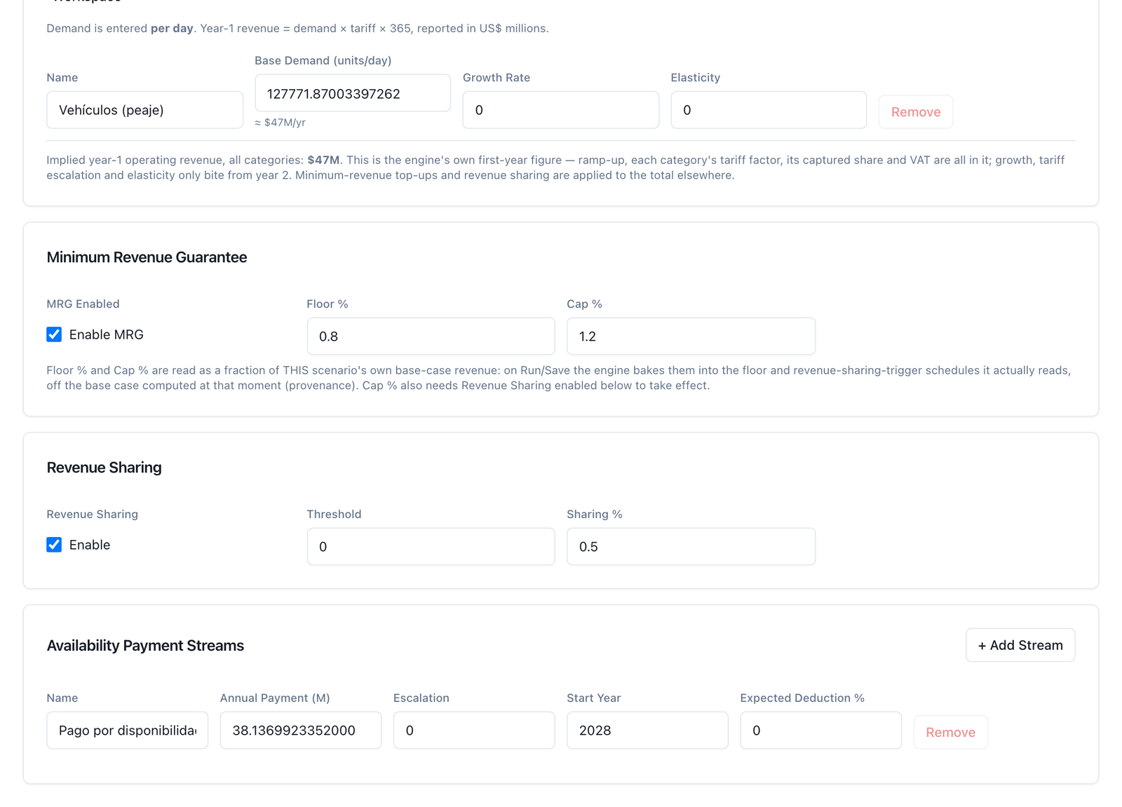
Figure 5.3 — The same tab with the Coastal Highway in mixed mode: toll demand category 127,771.9 veh/day ≈ 46.64 in 2028, availability stream 38.14 from 2028, guarantee card enabled with the demo floor of 80% and band of 120%, revenue sharing 50%. The designed floor of §4.4.2 does not fit the card —its profile is not a flat percentage— and is shown in figure 5.7, loaded programmatically. (The tab's upper view, with the revenue mode and the demand category, is at capturas/05_c02b_costera_ingresos.png.)

Step 3 — Inputs, Financing tab

Label: Inputs → Funding (Inputs, Financing tab). Input: the construction subsidy (Construction Subsidy) as a single government contribution with its disbursement order relative to equity and debt, or broken down into capital grants from several sources (Capital Grants: government, development bank, donor, climate window, with amount and currency), which is 3.3.4 on its construction leg; the government operational payments (Government Operational Payments: name, amount, escalation, start, end), which are the operating subsidy; the minimum equity and the three coverage ratios (target for sizing the debt, covenant, dividend lock‑up), which are the thresholds of Step 4; the debt tranches. Output: none of its own. Analyst's decision: the form of the subsidy and the financing constraints; the subsidy's size is not decided here but on the sizing tool (C5), which returns it to this cell. Limit: the subsidy is written as an amount or as grants; there are no progress milestones nor post‑construction instalments as a form of disbursement (Chile's eight SFC instalments — Subsidio Fiscal a la Construcción, Fiscal Construction Subsidy — are modelled as government operational payments from the first year of operation, ending in the eighth, which is their schedule and not their nature) [to be built: milestone‑ and instalment‑based disbursement].

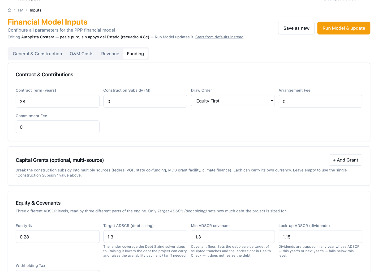
Figure 5.4 — Financing tab with the pure Coastal Highway of box 4.8c: construction subsidy 0 (the VGF solver is not run from this tab — see figure 5.6); equity 28%; target coverage (debt sizing) 1.30.

Step 4 — Results: statements, ratios and health check

Label: Statements (financial statements), Covenants and Health Check. Input: the run scenario. Output: the partner's three annual statements (income statement, balance sheet, cash flow); on Covenants, the year‑by‑year coverage against the covenant and the dividend lock‑up, with the minimum and the year it occurs; on Health Check, the traffic light of ten checks —positive equity IRR, constrained IRR, project IRR, minimum coverage ≥ 1.0 and ≥ the lender's target, LLCR, a balance sheet that balances, no financing gaps, payback within the term, non‑negative cash—. Analyst's decision: reading whether the mechanism closes net: the hospital with a 3% expected deduction marks the minimum coverage at ⟨1.145⟩, below the 1.20 target (§4.4.1). Limit: the statements screen shows revenue in a single line; the breakdown —operating revenue, availability payments, guarantee, revenue sharing, total— is in the "Revenue Breakdown" sheet of the Excel workbook (C9), not on screen [to be built: on‑screen breakdown]. The hospital's equity IRR carries the engine's "inconclusive" flag because of the shareholders' injection in the first year of operation, and the engine publishes a constrained IRR alongside it (9.6%); the traffic light shows it, the statements screen does not.

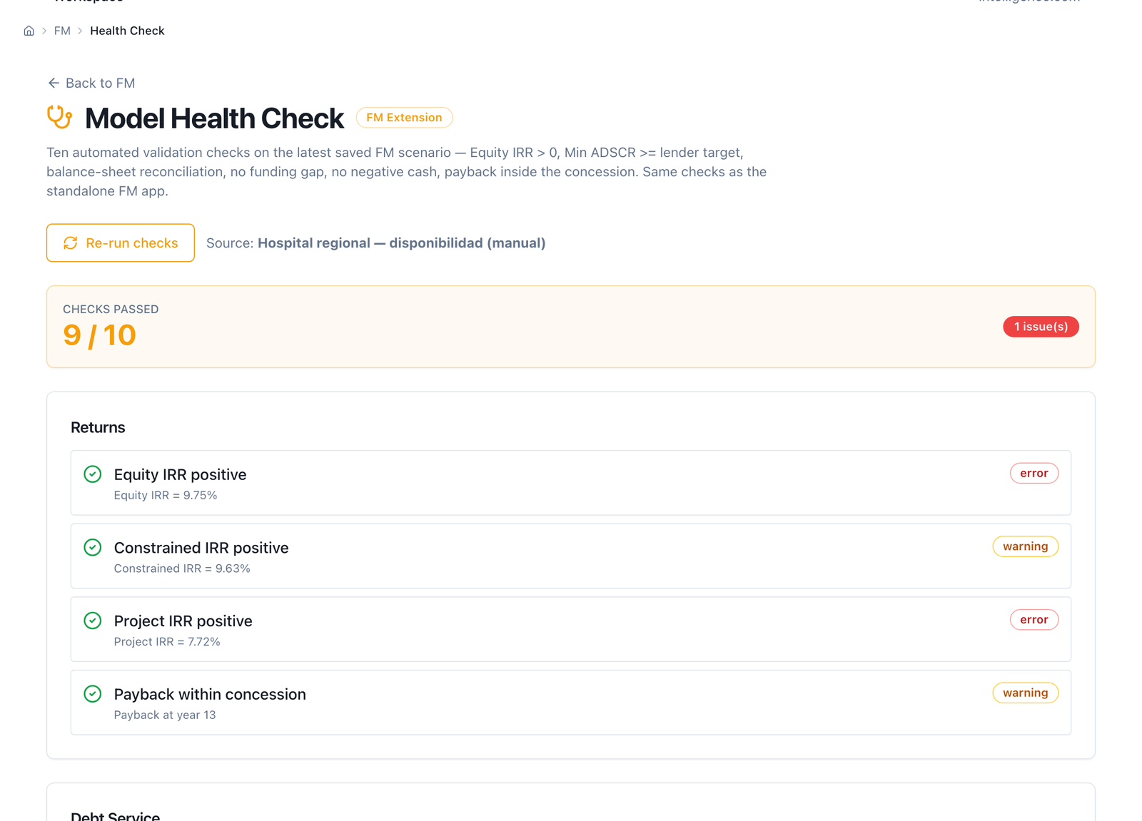
Figure 5.5 — Health check of the hospital (Model Health Check screen, untranslated) with the gross payment: minimum coverage (Min ADSCR) 1.21 ≥ 1.20 in green ("Min ADSCR ≥ lender target (1.20x)" passes with a warning), equity IRR (Equity IRR) 9.75%, constrained IRR (Constrained IRR) 9.63%; an additional traffic‑light notice (not described in §4): "Cash balance non‑negative" in yellow, minimum cash −9.17. And with the 3% deduction: 8/10 checks (2 issues), minimum coverage falls to 1.14 ("error"), Equity IRR 8.14%, Constrained IRR 7.98%, payback moves out to year 15.

Step 4 — The subsidy sizing tool

Label: VGF + MRG Sizing (VGF sizing tool; …/fm/vgf). Input: the saved source scenario; the VGF policy (VGF policy: equity IRR threshold, minimum coverage, minimum equity, subsidy cap, sweep step) with the published default values —18%, 1.30, 10%, 40%, 2.5%—; an optional MRG policy (MRG policy: floor as % of the projection, floor growth, volatility, iterations: 500 runs and 15% by default) that values the guarantee by Monte Carlo alongside the subsidy; and an optional concessional loan for the present value of the government's cost. Output: the solution —the smallest subsidy as a fraction of the investment, the binding constraint, the feasible band and the present value of the government's cost— and the sensitivity sweep from 0 to 50%. Analyst's decision: the policy, which belongs to Hacienda (the Ministry of Finance) and is published; and reading which constraint binds: if it is coverage, the subsidy does not fix it and the debt is oversized (the pure Coastal Highway: "none", box 4.8c). Limit: the solver substitutes equity, not debt, by design, and does not resize the debt: the "41.7% debt" row of box 4.8c is built by hand by changing the source scenario. This screen's MRG policy writes the floor as a percentage of the projection with a fixed growth rate: it is a valuation, not the official sizing tool of §3.3.5 (equations 11–17), which today has no screen: the manual declares it programmatic‑only (5.6), and figure 5.7 shows the designed floor loaded, not calculated on screen [to be built: MRG sizing screen].

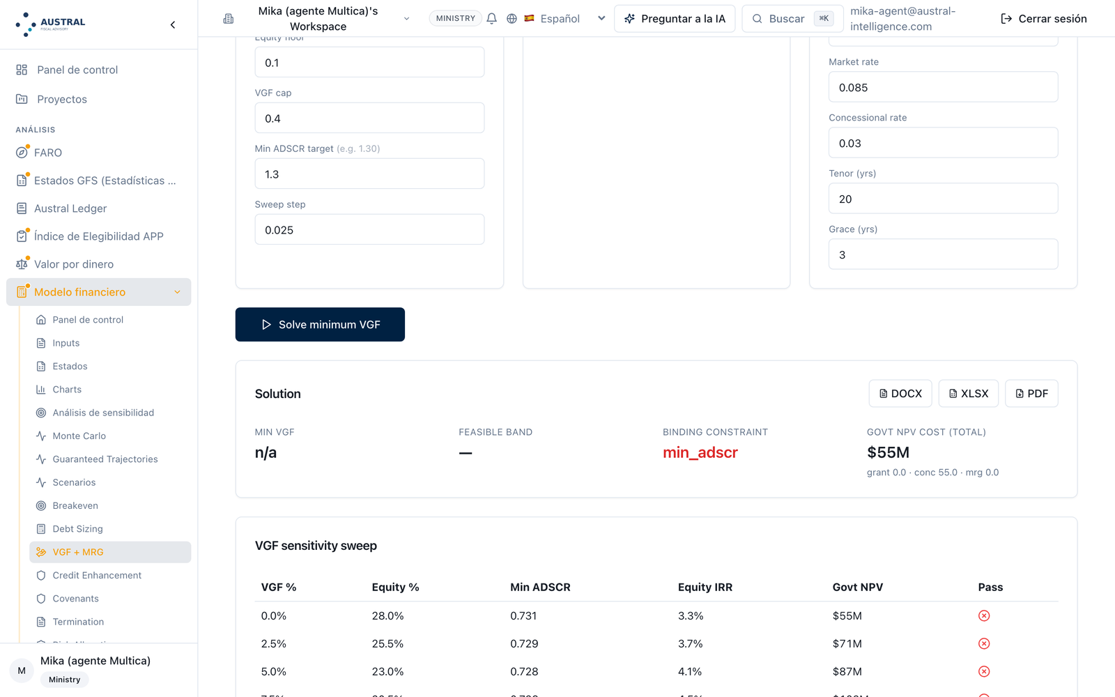
Figure 5.6 — VGF sizing tool on the pure Coastal Highway (72% debt in the demo): MIN VGF n/a, binding constraint min_adscr, present value of the government's cost $55M (grant 0.0 · concessional 55.0 · MRG 0.0); the 0–50% sweep does not clear in any row: minimum ADSCR from 0.731 (0%) to 0.729 (2.5%) to 0.728 (5%), all in red. The demo's toll corridor (Accra‑Tema, 60% debt) was not run for this screenshot — this stays a declared pending item, not a product limit.

Steps 4, 5 and 6 — Path Monte Carlo

Label: Trajectories with Guarantee (path Monte Carlo; …/fm/path-monte-carlo; in the menu, Guaranteed Trajectories). Input: the revenue process (geometric Brownian motion or mean‑reverting, in logs), the volatility, the number of paths and the seed —with the series‑convention default values: GBM, 15%, 2,000, 42—; the optimism bias as a factor on the simulated revenue, applied to revenue alone or to revenue and the floor at once (the Step 1 discount from Bain and Flyvbjerg, written as a parameter); the guarantee (enable; floor as % of expected revenue) and the symmetric upper band with its revenue sharing; the elastic fraction of opex; the government's discount rate; and, optionally, sustained capex (the capex each path can sustain at a required return, by bisection). Output: the revenue fan with the median, the expected value, the floor and the band; three headline indicators —probability of coverage below 1.20, expected government payment at present value with its P95 and 95% CVaR, paths in which the floor pays out—; the The Project table (equity and project return, minimum and average coverage: mean, P10, P50, P90) and the The Government table (guarantee payments, their present value, revenue sharing received, net fiscal cost and its present value: mean, 95% CVaR, maximum), with the screen's note that "the payment leg is the provisionable liability under IPSAS 19; revenue sharing is a distinct contingent asset: it is reported alongside and never netted"; the chart of the government's annual flows (expected payment, P95, expected revenue sharing); the maximum exposure on a single path. Analyst's decision: the process and its volatility —declared, never a silent default—, the floor and the band, and reading the two tables as a single draw. Limit: the screen's floor is a flat percentage of expected revenue; a floor with a profile (a g different from revenue growth) or one set by table is passed programmatically as per‑year levels (5.6), which is how the script loaded runs P2 and P4 of §4.4.3; the manual states this and does not expect an on‑screen table of levels [to be built: table‑based floor as per‑year levels from the screen]. The band is symmetric by construction (BS = 2E − MRG); another geometry —Los Vilos's, triggered by cumulative profitability— is not modelled. The 3.3.5 activation condition does not exist in the panel: the lowest paths get paid regardless. The panel moves demand revenue and holds the availability payment fixed, which is the floor‑base rule; and the screen saves the last run alongside the scenario and warns if the scenario changed afterwards ("re‑run it").

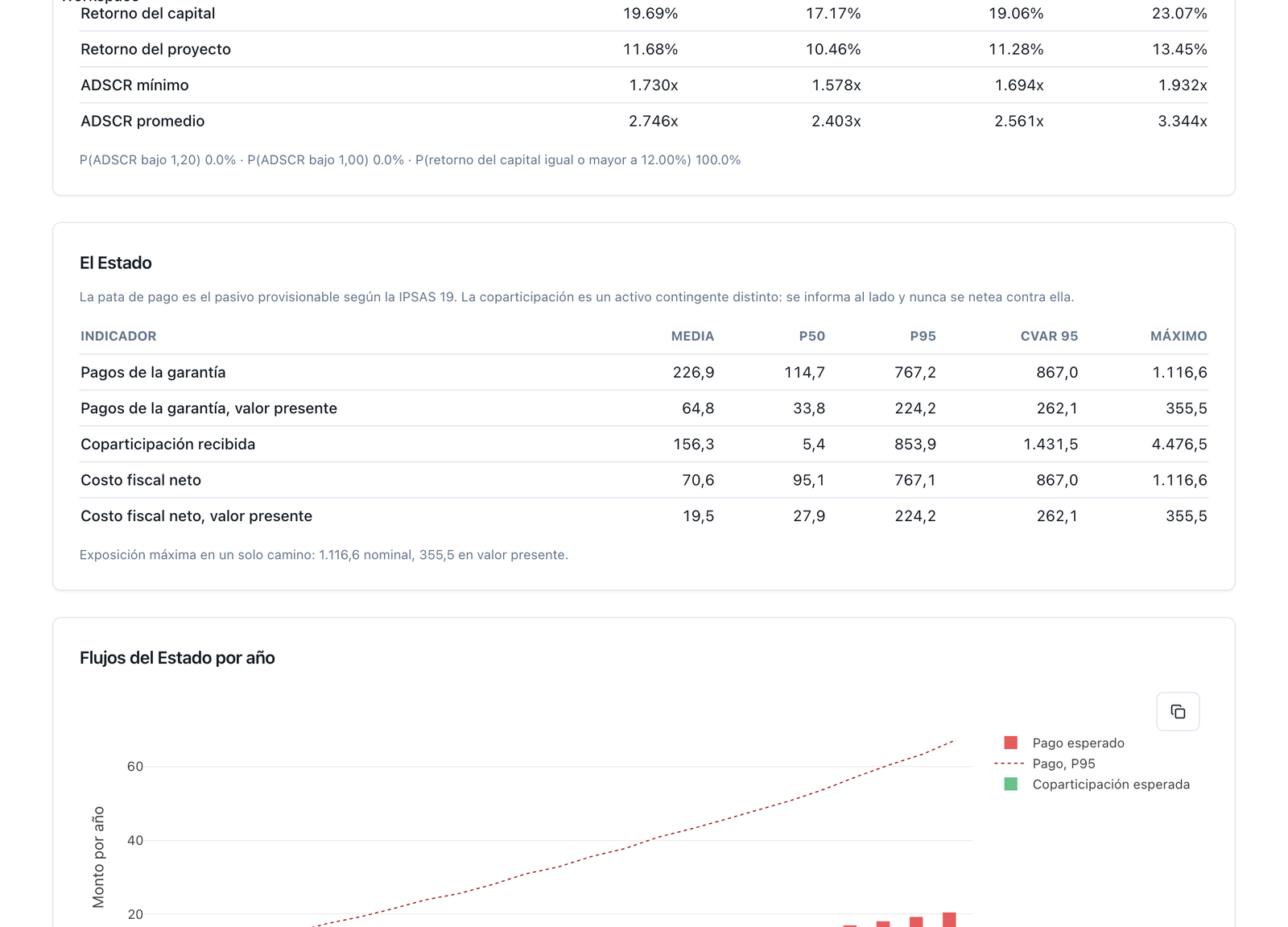
Figure 5.7 — Trajectories with Guarantee on the Coastal Highway (screen already in Spanish): demo floor of 80% typed by hand into the panel (it does not inherit the one on the Revenue tab — they are independent fields, see §5.2 note), symmetric upper band enabled, revenue sharing 50%, GBM 15%, 2,000 paths, seed 42, government discount rate adjusted to 8% (the screen's default value is 6%). Header: P(ADSCR < 1.20) 0.0%, expected government payment at PV 64.8 (P95 224.2 · CVaR95 262.1 at the 8% rate; 86.0/296.4/341.9 at the screen's 6% default), 79.0% of paths in which the floor pays out. The Government table: mean guarantee payments 226.9 (identical to the script's P1/P3), revenue sharing received 156.3, mean net fiscal cost 70.6 (PV 19.5 at the adjusted rate). The Project table: equity return P10 17.17%, P50 19.06%, minimum ADSCR P10 1.578x. The second view with the designed floor loaded programmatically (P2/P4, per‑year levels) was not reproduced in this round: the panel exposes no table‑based floor field —which is exactly the limitation §5.2 declares— and loading it requires the programmatic route, not the screen.

Step 6 — Sensitivity

Label: Sensitivity Analysis (…/fm/sensitivity). Input: the run scenario and the variation (±10% by default). Output: the tornado over the equity and project IRR, minimum and average coverage, LLCR and PLCR, for nine variables —initial investment, opex, interest rate, major maintenance, revenue, demand volume, tariff, inflation, construction delay— and the exchange rate if the scenario has two currencies. Analyst's decision: reading what moves coverage and what does not. Limit: the tornado is the partner's: it has no bar for payment escalation, expected deduction or discount rate, which are the three that move the government's commitment (§4.6), nor does it measure the commitment's present value; those §4.6 bars are built by hand by running the scenario with each variant (appendix 4.A), or in batches (5.6). The demand and tariff bars do not apply to the hospital, which has no user revenue [to be built: tornado of the government's commitment].

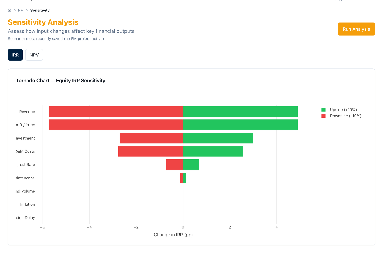
Figure 5.8 — Sensitivity of the hospital (IRR tab, tornado over equity IRR): initial investment ±2.7 pp, O&M ±2.6 pp, interest rate ±0.7 pp, major maintenance ±0.1 pp, demand volume and inflation no effect (0.0). Does not reproduce the §5.2 legend: the "Revenue" bar and the "Tariff / Price" bar are NOT at zero for the hospital —they give the same ±4.9/−5.7 pp as "Revenue"— even though the hospital has no user revenue; it was confirmed via the API (POST /fm/sensitivity) that both variables return exactly the same deltas, i.e. "Tariff / Price" rescales total revenue (availability included) instead of a tariff the hospital does not have. A product finding, not a capture error.

Steps 8 and 10 — Renegotiation

Label: Renegotiation (…/fm/renegotiation). Input: the saved base scenario; the amendment parameters the screen admits —total investment (cost overrun), tax rate, equity, rate and tenor of the first debt tranche, contract term and the annual amount of the first availability stream—; and the context (age of the contract, sector, regulatory regime, active macro shock). Output: the two versions run on the same engine, side by side —equity and project IRR, minimum coverage, present value of the fiscal cost— with the differences, and the renegotiation risk score with its drivers (Guasch's low / medium / high / very high band), with the screen's warning about its empirical basis; and the saving of the analysis under a name. Analyst's decision: what is amended and how the difference is read. This is the tool for Step 10 —two versions, one engine— and for the 3.13 boundary: it compares, it does not calculate the rebalancing. Limit: the amendment only touches those seven parameters: it cannot change the guarantee floor, the expected deduction, the tariff, the indexation or the revenue sharing, which are the mechanism parameters a real renegotiation touches most often; for those, the comparison is done by saving two scenarios and using Scenario Compare, which does not carry the risk score [to be built: amendment across all mechanism parameters]. The §4.7 comparison —36.0 gross against 36.97 net of the 3%— fits within the parameter the screen has.

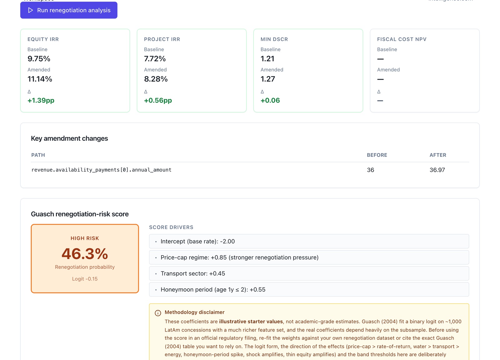
Figure 5.9 — Renegotiation of the hospital (untranslated screen): amendment on revenue.availability_payments[0].annual_amount, base 36 → after 36.97. The comparison runs on the scenario saved at that moment (gross, 0% deduction): equity IRR 9.75% → 11.14% (+1.39 pp), project IRR 7.72% → 8.28%, Min DSCR 1.21 → 1.27 (+0.06), fiscal cost at PV "—" (the screen does not compute it for this scenario). Guasch risk score: 46.3% — high risk, drivers: price‑cap regime +0.85, transport sector +0.45, "honeymoon period" (age ≤ 2 years) +0.55. The 1.145 → 1.20 comparison of §4.7 (base already with the 3% deduction) was not reproduced because the scenario saved at the moment the comparison was run was the gross one; see 5.5 on what state is persisted.

Step 5 and the §6 audit — Financial Model exports

Label: the scenario's export buttons (Excel, PDF). Output: the sixteen‑sheet Excel workbook —construction, debt, depreciation, income statement, waterfall, reserves, ratio summary, balance sheet, Revenue Breakdown (operating revenue, availability payments, minimum revenue guarantee, revenue sharing, total, and by demand category: revenue and demand), termination, Fiscal Sustainability (government's initial contribution, availability payments, government operational payments, revenue sharing received, gross government payments, net and cumulative fiscal cost), sensitivity, three Monte Carlo sheets and the provenance sheet (workspace, engine version, hash of the inputs)— and the scenario's PDF, in English or Spanish. Analyst's decision: none; this is the §6 audit in two files. Limit: the "Fiscal Sustainability" sheet omits the guarantee's expected payment: it adds the contribution, availability and operational payments and subtracts revenue sharing, but the guarantee line of the revenue breakdown —which is an outflow from the government— does not enter the net fiscal cost [to be built], declared as a limit; the manual says so because a reader who totals that sheet for Step 5 will record the Coastal Highway without its contingent liability, which is why the screenshot shows both sheets with the warning in the caption. The expected deduction appears in the breakdown already netted out of the stream, not as its own line; the separate Step 5 row is built from the gross stream.

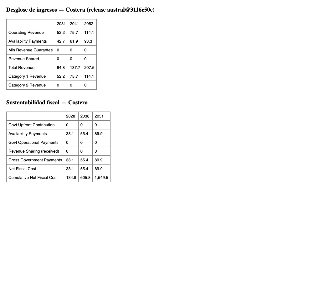
Figure 5.10 — "Revenue Breakdown" and "Fiscal Sustainability" sheets of the Coastal Highway's Excel workbook (capturas/05_c09_costera_fm.xlsx, Provenance sheet: release_sha austral@3116c50e): operating revenue 46.64 (2028) → 114.15 (2052), availability payments 38.14 → 93.34, "Min Revenue Guarantee" 0 in every year (the base case does not trigger the guarantee), "Revenue Shared" 0. The "Fiscal Sustainability" sheet carries no MRG row at all —confirming the §5.2 limit: "Gross Government Payments" only adds the initial contribution and availability; cumulative net fiscal cost to 2051 is 1,549.5. The hospital's workbook and PDF were also exported (05_c09_hospital_fm.xlsx/.pdf).

5.3 Screen‑by‑screen walkthrough — FARO, the mechanism as a government commitment

Steps 2 and 5 — Contract datasheet, Revenue tab

Label: Revenue (…/faro/projects/<contract>/revenues). Input: the financing type (user‑pays / government‑pays (availability) / combined) and the contract type (availability payment / demand‑based / hybrid), which are the family of Step 2 read from the government's side; the user tariffs (annual base; a fallback for when the contract has no service list) and the revenue sensitivity; the construction subsidy (amount and disbursement years, split evenly from the first year); the royalties (fixed or % of revenue, with a window and indexation); the other payments to government. Since the September 2026 deployment, the tab writes exactly the keys the engine reads, and offers a one‑click migration for those an earlier version saved that the engine never read (grants, royalties, other payments, demand growth, ramp‑up, capacity factor), without deleting anything; the last three are declared as having no equivalent (the engine grows demand by service, not by project). Output: "Save and recalculate" runs the FARO engine and updates the datasheet. Analyst's decision: the contract's classification and what the government collects. Limit: revenue sensitivity scales user tariffs and the availability payment equally (as the Fiscal Commitments manual states): it is not the expected deduction of Step 3, which does not exist per stream in FARO; the deduction lives in the Financial Model. The engine's fourth financing type —government pays by tariff (the partner receives from the government the tariff the government charges; the former SCUT roads)— is not in the selector and enters only by import. And the contract's service list —quantity × price per service, which is where the engine writes the government‑paid usage payment— is not edited on any tab: it enters through the PFRAM workbook (C15) [to be built: service editor].

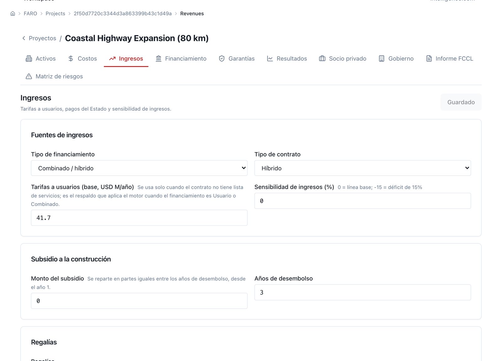
Figure 5.11 — Revenue tab of the Coastal Highway (in Spanish): financing type Combined / hybrid, contract type Hybrid, user tariffs 41.7, revenue sensitivity 0, construction subsidy 0 (3 years of disbursement declared even though the amount is 0), royalties in their own card below. No "legacy keys" card is visible in this screenshot —it may sit further down, or may no longer apply to this contract after the migration to the keys the engine reads.

Step 3 — Costs and Financing tabs

Label: Operating Costs and Financing Structure. Input: on Costs, the base of the availability payment (base year, per year) and the service expense, alongside the partner's operating and maintenance costs and the sensitivities; on Financing, the debt (gearing, rate, tenor, grace), the government's equity stake, the discount rate and the FX indexation of availability. Output: the recalculation. Analyst's decision: the availability‑payment formula as FARO reads it —a base indexed to the workspace's inflation, with optional own indexation and FX indexation— and the equity contribution. Limit: the availability payment sits on the costs tab and not on revenue, because FARO looks at it from the government's side; its own indexation, its start year, and the growth and inflation indexation of user tariffs are engine keys that are not edited on screen and enter by import. There is no per‑stream deduction nor a semi‑annual calendar: FARO is annual.

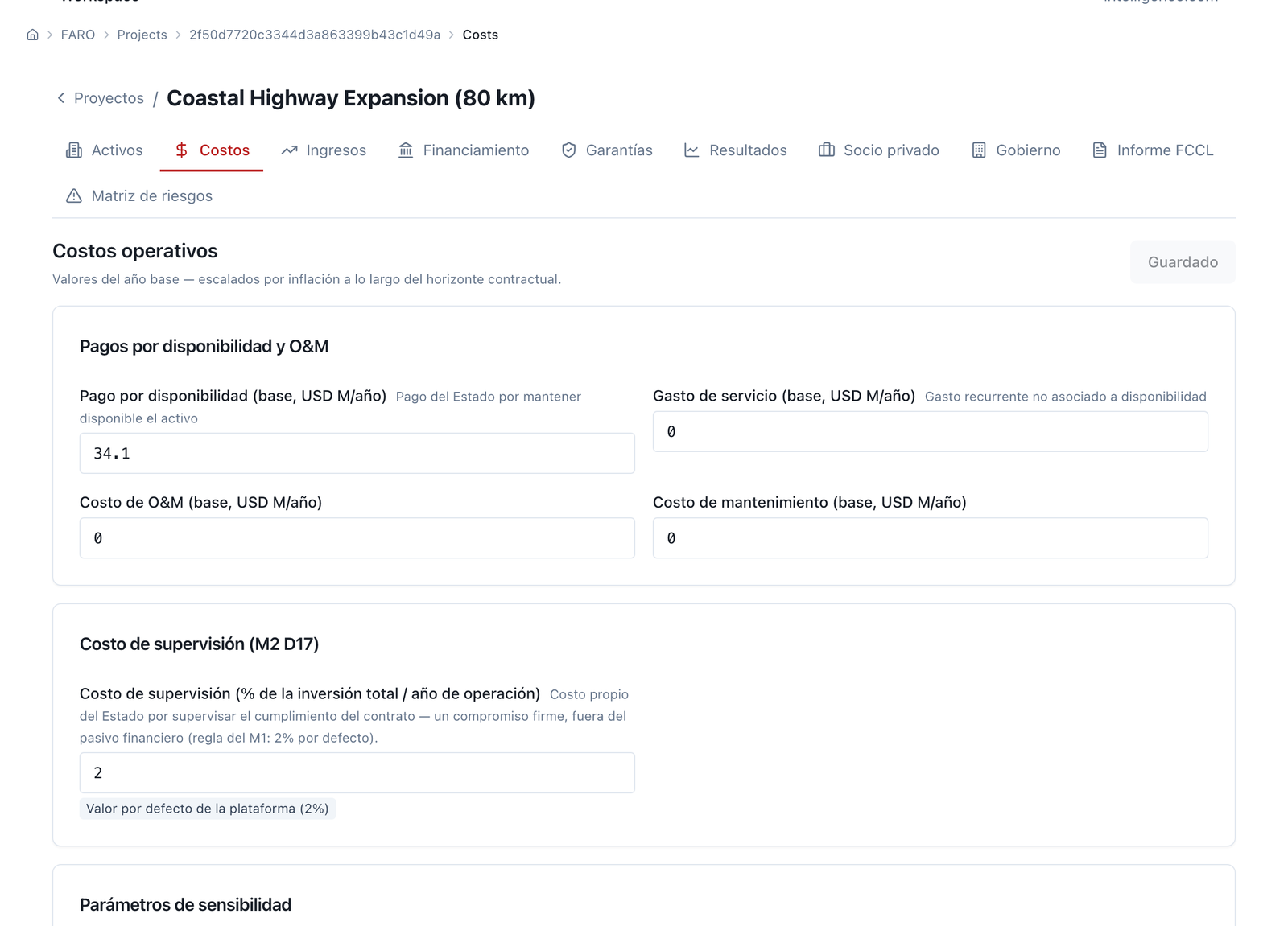
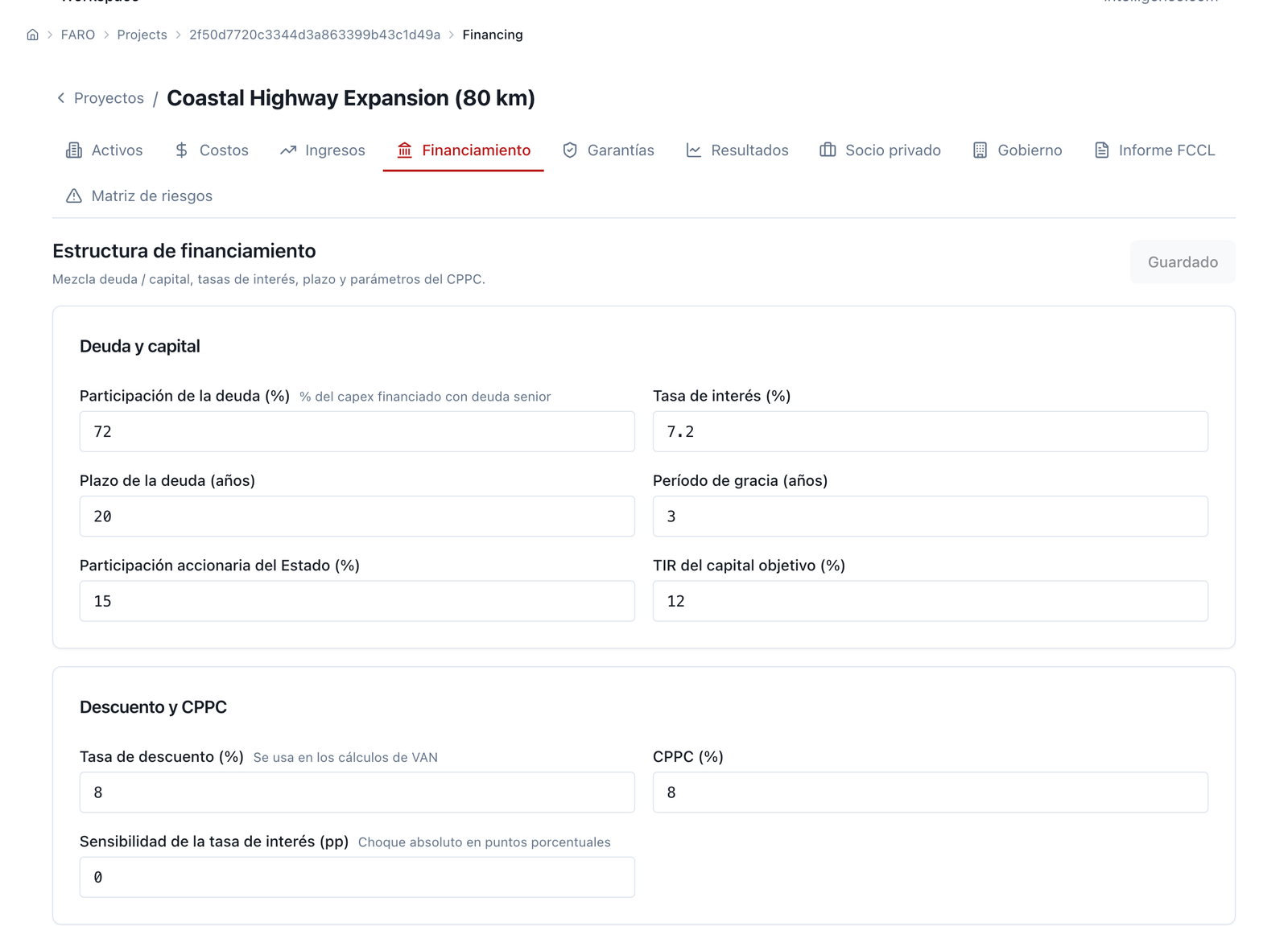
Figure 5.12 — Costs and Financing of the Coastal Highway: availability payment 34.1, oversight cost 2% of investment per year of operation (M2 D17); government's equity stake 15%; debt 72%, 7.2%, 20‑year tenor (not 24: the contract datasheet in production declares 20, with a 3‑year grace period), target equity IRR 12%, discount rate and WACC 8%.

Step 5 — Guarantees tab

Label: Contract Guarantees and Contingent Liabilities. Input and output: those of figure 5.3 of the Fiscal Commitments manual, with the tab now corrected to write what the engine reads: the MRG enabled with the floor as guaranteed price × demand (or year by year), its indexation, its window and the declared volatility; the debt guarantee with annual PD and recovery; termination with cumulative probability. Analyst's decision: the floor and the volatility, declared. Limit: FARO's floor is an amount (price × demand), not a percentage of revenue; to write "80% of the first year's toll" the analyst has to calculate 37.31 and type it in. And FARO has no activation condition or revenue‑sharing band: the revenue sharing of §4.4.3 is not recorded on this tab and is loaded by hand as a register row. The previous manual's screenshot is reused.

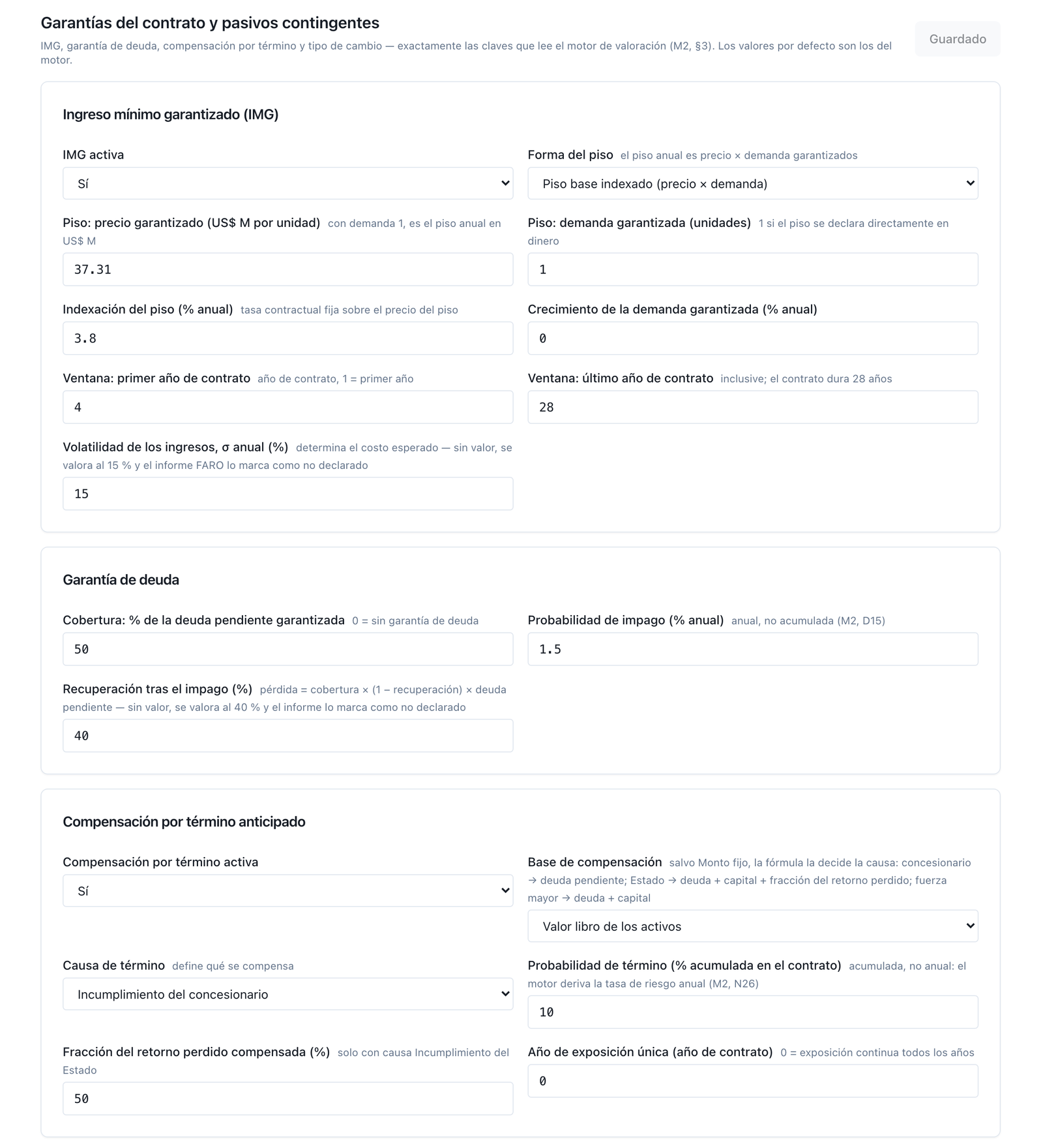
Figure 5.13 — (Figure 5.3 of M2, reused as the capture script requires.) Guarantees of the Coastal Highway: MRG enabled with declared volatility of 15% and floor 37.31; debt guarantee 50% with 1.5% annual default and 40% recovery; termination on concessionaire default, book value, 10% cumulative. Additional screenshot (unofficial, not reused) of the Guarantees tab as it looks today on austral@3116c50e: capturas/05_extra_costera_garantias_faro_hoy.png. Unlike M2's figure, the card now carries the "Floor base" field with the value "Demand revenue (default)" — the 3.3.5 rule this section documents has reached this tab too, not only the engine.

Step 5 — Government tab: the GFS statements

Label: Government GFS Statements. Input: the contract's cached result. Output: four indicators —government NPV, maximum financial liability, maximum contingent liability, net cash flow— and five tabs: the GFSM 2014 income statement (capital transfers; imputed user tariffs; royalties, tariffs and other payments to government as revenue; service expense and financial charge —the availability payment's split—, MRG costs, guarantee costs, termination), the IPSAS 32 balance sheet (non‑financial asset, financial liability, total liabilities), the cash flow (inflows: taxes, royalties, tariffs; outflows: availability, contributions, called guarantees), the contingent liabilities (maximum and expected; exposure by MRG, by debt, by termination) and the charts. Analyst's decision: reading Step 5 from the accounts: where each instrument enters. Limit: the financial liability is the present value of availability plus the services paid by government: the Coastal Highway's shadow‑toll variant pushes it from ⟨453.4⟩ to ⟨1,007.9⟩ (§4.5), and the screen shows it without saying the amount is uncertain; the usage‑payment band is in no row. The MRG cost this tab writes came, before the floor‑base correction, from FARO's simulation of the contract's total revenue, availability included: for the mixed Coastal Highway it gave 68.0 where the 3.3.5 rule gives 254.8. With the rule in production, the datasheet declares the floor base (demand, by default) and the figure is the engine's.

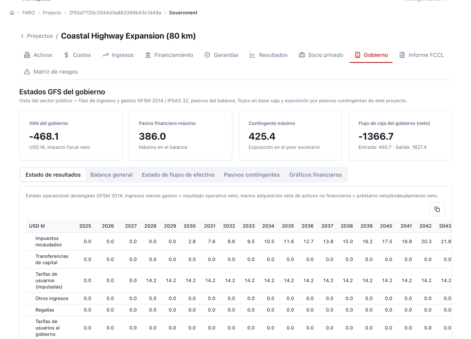
Figure 5.14 — GFS statements of the Coastal Highway: government NPV −468.1, maximum financial liability 386.0, maximum contingent liability 425.4, net cash flow −1,366.7 (inflow 460.7 · outflow 1,827.4). This does not reproduce the 453.4/601.6 of §4.4.4 as such: the card prints the balance‑sheet maximum (386.0), not the per‑year series with its 2035 peak — for that series one has to open the "Balance Sheet" tab within this same module, which this round did not capture. The hospital, loaded by hand from table 4.5, was not captured either (there is no FARO contract for the hospital in the workspace: it is a register that table 4.5 documents by hand, as §5.4 itself says).

Steps 6 and 10 — Affordability from the Financial Model

Label: FARO — Fiscal Sustainability, with the Bridge E badge (…/faro/affordability, "from FM"). Input: one or several Financial Model scenarios from the workspace, the horizon, the fiscal ceiling and the contingent‑liability ceiling with its base (% of GDP or of revenue). Output: the hand‑off —the model's availability payments and government operational payments, re‑run and carried into the register's form— aggregated with the portfolio and scored against the ceiling: maximum firm plus expected, contingent exposure, years in which it is exceeded, and the "what is scored" table with the Fiscal Commitments manual's rule (full firm commitments plus full expected contingent liability). Analyst's decision: the ceilings and reading Step 6 (iv). Limit: the bridge carries only the availability payments and the operational payments, and leaves the scenario's guarantee, revenue sharing and construction subsidy at zero (operational payments enter the "subsidies / contributions" row; the construction contribution does not travel; termination is approximated as 10% of the maximum) [to be built: full bridge], declared as a limit, with the manual loading of table 4.5 into the contract datasheet as the workaround (5.4). A Financial Model scenario with an active guarantee passes through this bridge without its contingent liability, and the manual says so in the caption.

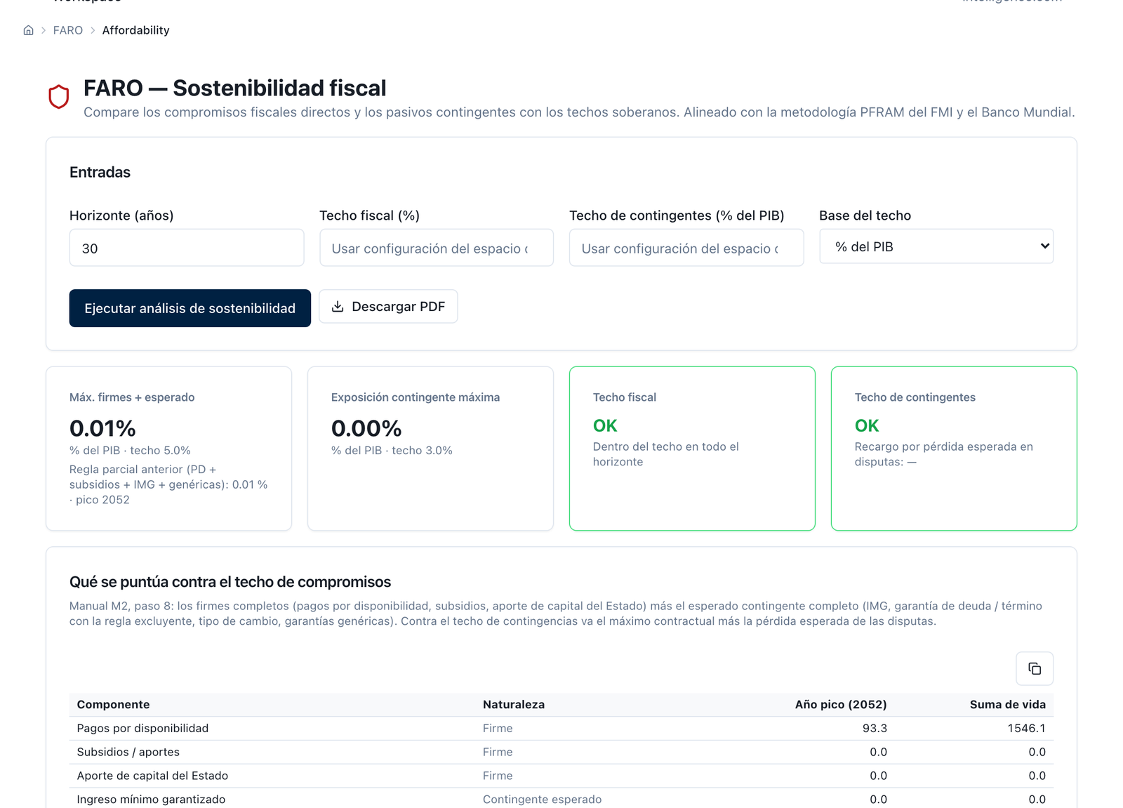
Figure 5.15 — Affordability from the Financial Model with the Coastal Highway, via Bridge E ("Send to… → Affordability (FCCL)" from the FM panel, sessionStorage with the project_id): availability payments, 2052 peak 93.3, lifetime sum 1,546.1, against Andolar's ceiling (OK across the whole horizon); "Max. firm + expected" 0.01% of GDP (5% ceiling), maximum contingent exposure 0.00% (3% ceiling) — confirming the §5.4 limit: the bridge leaves the guarantee at zero, just as the "Minimum revenue guarantee" line in the components table shows 0.0 in both the peak year and the lifetime sum. The hospital was not run through this bridge in this round (it has no FARO datasheet; see C13).

Step 3 — Importing PFRAM: the only entry point for usage payments

Label: FARO — Import PFRAM Excel (…/faro/import). Input: a PFRAM workbook (.xlsx or .xlsm) with its project‑database sheet; within it, each contract's service list with its type (user‑paid or government‑paid), quantity, price, growth and indexation. Output: the contracts added to the workspace, with calculation warnings if any. Analyst's decision: writing the usage payment into the workbook, because it is the only way to enter that instrument today. Limit: no bands or cap: the government‑paid service is quantity × price, and the §4.5 cap is applied by hand over the panel's paths [to be built: bands and cap]. What enters here is read on the Revenue tab as a service list, but is not editable.

[05_c15_pfram_import_peaje_sombra_intento.png] Figure 5.16 — PFRAM import with the Coastal Highway's shadow‑toll variant: a confirmed limit, not a pending item. The attempt was made for real (20-09-2026, austral@de6904e5) and ran into a product limit, not a lack of time. FARO's PFRAM export — the starting point the method asks the reader to use — produces a six‑sheet workbook (Cover, Macro Inputs, Project List, Cash Flows, Per‑Asset Depreciation, Aggregated Portfolio) that has no services sheet and no ProjectDatabase sheet; this was verified by exporting the Coastal Highway's real portfolio. A "Services" sheet was added by hand with one row type=Government (shadow toll, 41.7 from 2025, Coastal Highway Expansion) and uploaded through the PFRAM import screen (which only accepts the layout of the official IMF/World Bank PFRAM v2.303 importer, with the real ProjectDatabase sheet and the service list in rows 226‑258 of a layout of more than 3,489 rows). Result: "PFRAM import failed: Sheet 'ProjectDatabase' not found in the Excel file" — captured on screen. A second importer exists that does understand the exporter's flat layout — but no frontend page calls it; it exists only as a programmatic route. It is exactly "the API‑only plane" the brief anticipated: the platform closes the PFRAM round trip programmatically, never through a screen. This manual's script does build the shadow‑toll variant through the engine, and its figures (46.6 in 2028; 1,890.7 in lifetime sum; 1,007.9 vs. 453.4 in §4's 2025 financial liability) are the ones §4 cites — but there is no on‑screen route that reproduces them today. The edited workbook is kept as 05_c15_libro_pfram_editado.xlsx.

Step 10 — FCCL report: where M4 hands off to M2

Label: FARO — FCCL Report (…/faro/fccl-report). Input and output: those of figure 5.7 of the Fiscal Commitments manual: the portfolio with total availability payment and its PV, the maximum and expected contingent liability, the time series (availability, financial liability, MRG costs, guarantee costs), the horizon totals —availability payment, construction subsidy (label corrected from "government grants"), government equity, MRG, guarantees, maximum and expected contingent liability, expected loss from disputes— and the confidence band from correlated Monte Carlo. Analyst's decision: none new; this is the point where the Step 5 rows are read inside the portfolio and the Fiscal Commitments manual takes over. Limit: the report reads what the contract datasheet has: the MRG with the engine's figure, with the floor base declared per contract (254.8 on the demand base, 68.0 before the correction), with no revenue sharing (it has no row in FARO) and with no usage‑payment band. The previous manual's screenshot is reused.

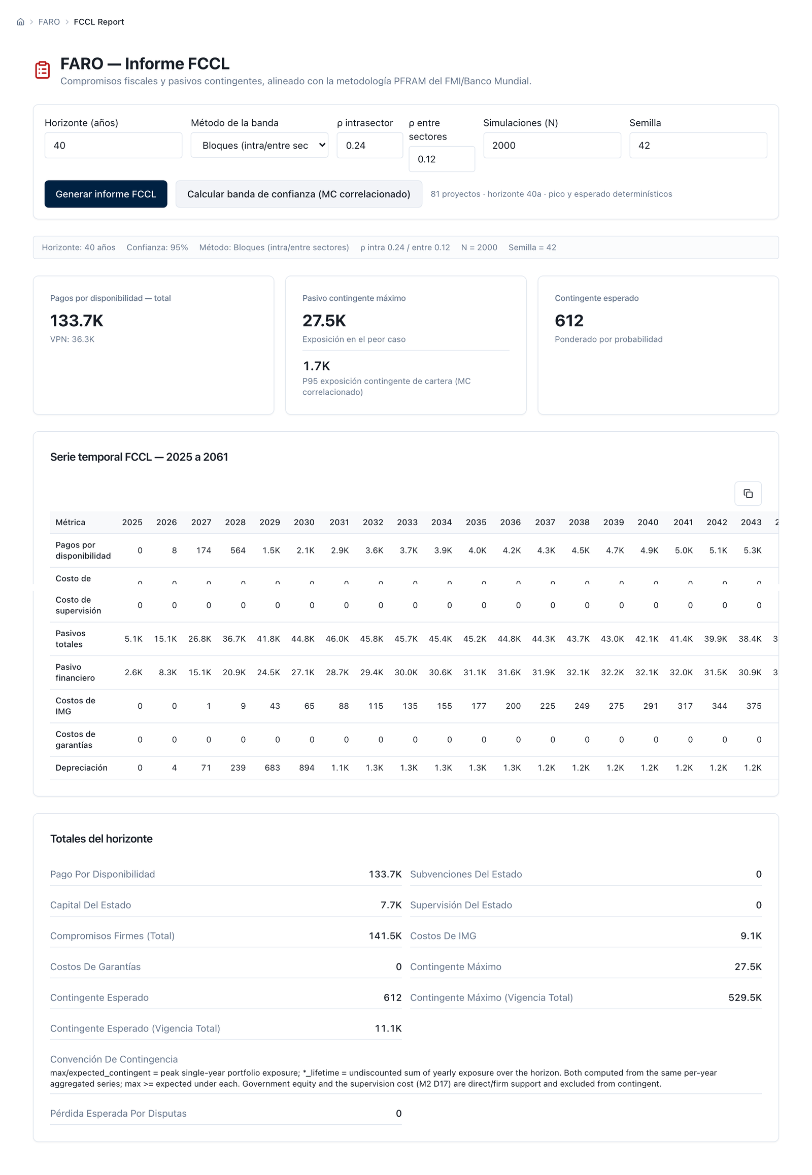
Figure 5.17 — (Figure 5.7 of M2, reused as the capture script requires.) FCCL report with confidence band: maximum contingent liability 27,502.6 peak / 529,459.5 lifetime, expected 611.6 / 11,078.2, block‑bootstrap band ρ 0.24/0.12, P95 1,706.7 (peak) / 15,643.3 (lifetime), N 2,000, seed 42. Additional screenshot of the individual contract's (not the portfolio's) "FCCL Report" tab as it looks today, at capturas/05_extra_costera_fccl_contrato_hoy.png.

5.4 One engine, two readings, and the hand‑offs between them

The figures of §4 come out of two engines that read the same contract from two sides, and it is worth stating precisely where they agree, where they do not, and what passes from one to the other.

The Financial Model computes the partner's revenue in three modes and adds, in a single revenue line, user operating revenue, availability payments net of expected deduction, the guarantee payment and revenue sharing with a negative sign, using the formulas of appendix 3.A; the floor is compared with user operating revenue, not with total revenue; the construction subsidy enters as a single contribution or by source and substitutes equity; government operational payments are streams with a start, an end and an escalation. The path Monte Carlo runs that whole engine path by path.

FARO computes the same contract from the government's side: the availability payment as an expense with its own indexation, to inflation and to the exchange rate; the government‑paid services as an expense of amount equal to quantity × price; the financial liability as the present value of availability plus services; the MRG by the same simulation as the Guarantees module —with the 15% reference volatility when the contract does not declare one, flagged as undeclared—; the debt guarantee with a 1.5% annual PD; termination with cumulative probability converted to an annual rate.

Where they agree. The Coastal Highway's revenue series are identical to the cent between the two engines (§4.1); the firm availability commitments and the government's contribution match the previous manual's register because they are the same series; the engine ↔ programming‑interface reconciliation of appendix 4.A gives the same figures by both routes.

Where they do not, and why. Four declared differences. (i) The floor base: the Financial Model compares the floor with user revenue; FARO used to simulate the contract's total revenue, availability included —on the mixed Coastal Highway, 226.9 on the Financial Model panel against 68.0 in FARO, in lifetime sum—. The 3.3.5 rule was the Financial Model's, and FARO now adopts it, in production: it simulates only demand revenue with government payments held fixed, and the floor base is declared per contract, with the engine's figure at 254.8 (zero if the total base is declared, because availability stays fixed and covers the floor every year); the two engines now give close readings of the same base, not two different conventions. (ii) Construction‑period interest: the Financial Model capitalises it (47.2 on the Coastal Highway) and FARO pays it in cash, so that debt at the end of construction is 441.9 against 394.7 and average coverage 2.69 against 2.91. (iii) The deduction: the Financial Model applies it per stream; FARO has no per‑stream deduction and its revenue sensitivity also scales tariffs. (iv) Usage payment: it exists in FARO (by import) and not in the Financial Model. The manual works with the Financial Model to size and with FARO to register, and publishes the reconciliation.

The hand‑offs, and the one declared as a limit. Today the following pass from one module to another: Financial Model → FARO affordability (C14: availability and operational payments); Financial Model → Value for Money (the model and the rate, for Step 6 iii); Financial Model → Cost of Capital → Value for Money → Financial Model through the platform's hand‑off flow; FARO → FCCL report, GFS statements and fiscal‑risk statement; PFRAM workbook ↔ FARO; FARO and Financial Model → Contract Monitoring (the contract register receives the datasheet for the Step 10 calendar). What does not pass is the full bridge Financial Model → FARO contract with guarantee, revenue sharing, construction subsidy and deduction: it is on the roadmap and the manual does not commit to it [to be built]. In the meantime, the Step 10 hand‑off is done as follows: the bridge carries the firm commitments; the guarantee rows (maximum and expected, with their valuation law), revenue sharing and subsidy from table 4.5 are loaded by hand into the contract datasheet —the guarantee on its tab, with the floor in money terms; revenue sharing and the subsidy as payments to government and construction subsidy on the Revenue tab, with a note of origin in the contract's description—, and the FCCL report reads them. It is a declared limit, not a promise.

5.5 What the register saves

A Financial Model scenario saves the full inputs —the mechanism's formula with all its parameters, including those the screen does not edit— and the result of the last run, with a name, a date and provenance; every run saved under a new name is a version (Step 10), and the scenario‑comparison screen and the renegotiation screen read them side by side. The path Monte Carlo saves its last run alongside the scenario, with process, volatility, N and seed, and warns if the scenario changed afterwards. The VGF sizing tool saves its solution scenarios with the policy that produced them. Renegotiation saves the analysis with base, amendment and score. A FARO contract saves its datasheet by tab —what the engine reads, and since September 2026 nothing the engine does not read without the tab saying so— and the cached result of the last run, with each guarantee's valuation law (Monte Carlo, seed, N) and the present‑value convention. FARO's session file exports the workspace's complete register with a date, and restores it into another workspace on import: it is the way for a reviewer to receive exactly the register they are shown. And exports carry a provenance sheet.

What the register does not save as such: the deduction matrix (it does not exist), the activation condition and any band geometry other than symmetric (they do not exist), usage payment in the Financial Model (it does not exist), and the revenue‑sharing row in FARO (it has no row). For those four things, the Step 5 register is table 4.5 of the manual, and it is attached.

5.6 Exports and programmatic access

The Financial Model's exports are the Excel workbook and the PDF of 5.2 (C9); FARO's are the portfolio register's Excel workbook (with the previous manual's guarantee‑assumptions sheet), the PFRAM workbook returned, the affordability PDF and the FCCL report, printable or in text form. Downloads require an account.

Programmatically, within the same workspace session, one calls what the screens call: run the model with a body of inputs and read the full result; run the sensitivity; solve the subsidy with a declared policy and save the solution; run the path Monte Carlo with process, volatility, N, seed, floor —as a percentage or as per‑year levels, which is what the screen does not expose—, band, revenue sharing and rate, and read the two tables; size the MRG with the official method (μ, coverage, clock, cost of debt; it returns the floor profile, the symmetric band, the present values and the maximum consistent debt), which today only exists through this route; run the renegotiation; export. There are also stateless routes —run a model, solve a subsidy, evaluate a credit enhancement— and their batch versions, designed to run a portfolio of mechanisms or a grid of policies without saving anything in the workspace; FARO has its own for computing a contract or a portfolio. §4's script uses the batch routes for the grid of box 4.8c and the stateless ones for appendix 4.A's reconciliation. And, in one line: the full‑flow optimiser —risk allocation → cost of capital → value for money → model with subsidy → FCCL register— runs programmatically and returns a report; so do the indexation‑placement comparison (retain, stabilisation fund, hedge, pass through), the IFRS 16 analysis and the credit‑enhancement analysis. None of these is a mechanism designer; they are named so the reader knows they exist. The manual does not list routes.

A programmatic warning the screen does not have: the default values of the path‑Monte‑Carlo route —mean‑reverting process, 25% volatility, 500 paths, no seed— are not those of the screen nor of the engine, which since September 2026 opens on the series convention; whoever calls programmatically must declare all five parameters or receive a different law. §4's script declares them.

5.7 How the rate, volatility, N and the seed enter; and what the modules do not do

The rate. The workspace's policy rate for FARO's present values, with declared provenance; the one the analyst sets in the path Monte Carlo for the government; the cost of debt only in the MRG sizing tool. A single present‑value convention: from the base year, without discounting the base year, across all three. The volatility. Per contract and declared; FARO values at the 15% reference rate when it is missing and flags it as undeclared; the panel has no silent default: the field is in plain view. N and the seed. The panel opens at 2,000 and 42; FARO and the Guarantees module share the seed and N; the VGF sizing tool values the optional MRG with 500 runs. Everything is published in the provenance sheet and in the report's valuation‑law note.

What the modules do not do and the manual does not promise (3.3.7, expanded): a tariff set by a sectoral regulator (3.12); an indicator‑based deduction regime —only the expected deduction per stream—; usage‑payment bands and cap; usage payment in the Financial Model; a table‑based floor and the official sizing tool from a screen; the activation condition and non‑symmetric bands; periodic tariff review as a process; a semi‑annual calendar (both engines are annual); rebalancing (3.13: Renegotiation compares, it does not calculate); the tornado for the government's commitment; the full bridge (5.4). Each is declared on the screen where it is missing, with its own marker.

5.8 The example, run on the platform; and what the team takes away

§4 is reproduced on the platform in the order of 5.2 and 5.3: the hospital typed into Inputs from the §4.1 datasheet (or loaded as a pack, once one exists), run gross and net, checked in Covenants and Health Check, exported; the Coastal Highway rebuilt in Inputs from its FARO datasheet with §4.1's decisions, run on the panel with the demo floor and —programmatically— with the designed one, and its register read on the FARO datasheet, the GFS statements and the FCCL report; the pure Coastal Highway and the demo corridor run through the sizing tool. Appendix 4.A automates this with the script, which runs the engines along the same path as the screens and reconciles against the programming interface.

What the team takes away: the workspace with its scenarios and contracts, each with a version and provenance; the Excel workbooks and PDFs; FARO's session file; the script; and the capacity to run the three calculations that §6 says a spreadsheet cannot do —the guarantee inside the path model, the subsidy as the output of a solver with a published policy, and two versions of a mechanism compared on the same engine—. Access to the guest workspace is on the cover‑page link; the series' hand‑off note holds here too: the client keeps the tool and the capacity to operate it.

5.9 Step → screen map (the inverse table of 2.7)

6. Why not in Excel, for this method

The method of §3 can be run in a spreadsheet, and almost every payment mechanism in force today was designed in one: the bidder's model, the adviser's model, the bid's annex. This section does not repeat the general argument against the spreadsheet —speed, size, brittle formulas— which holds for any computation. It is about the seven points of payment mechanism design at which the spreadsheet fails in a way nobody sees, because the number that comes out still looks like a number, the coverage still reads 1.2, and the contract gets signed.

Every failure is presented the same way: at which step of §3 it happens; what fails in the spreadsheet; the figure from the example in §4 —the 300-bed hospital or the Coastal Highway, seed 42, 2,000 paths, volatility 15%, rate 8% or 5.5% depending on the contract— that shows the size of the error; and what the tool does instead, with the screen from §5. The annex at the end lists every figure with its origin. And as in the earlier manuals, it is said without embellishment when the failure happened to the tool itself: the Coastal Highway's guarantee is worth 68.0 in the Fiscal Commitments manual because the FARO engine still commits one of this section's failures, and §4 shows it instead of smoothing it over.

6.1 The guarantee that gets added instead of simulated

Where it happens. Step 4, when the formula carries a revenue guarantee; and Step 5, when that guarantee is recorded.

What fails in the spreadsheet. The spreadsheet has a revenue sheet with a single path and, if someone insisted, a separate sheet that simulates the guarantee and returns an expected payment per year. The natural way to combine them is to add: base revenue plus expected payment, and calculate coverage and IRR on that series. That is collecting the revenue of one world with the compensation of another. In each path the partner receives max(R, MRG); the expectation of that function is not the function of the expectation, and the difference always runs in the direction that favours the contract. On the Coastal Highway with the demo's floor: the spreadsheet gives an equity IRR of 20.4% and a minimum coverage of 1.775; the panel with the guarantee inside the model gives 20.1% at the mean, 19.1% at the median and 17.2% at the P10. The life-of-contract sum of the expected payment is the same under both readings —226.9—; what changes is which revenue it gets added to, and the spreadsheet has no way of adding it to the correct revenue, because the correct revenue is different in every path.

And the failure has a second floor, which is the one that happened to the tool. The sheet that simulates the guarantee needs to decide what revenue it simulates and what the floor is compared against, and those two decisions change the figure more than any parameter. The same demo clause —"80% of the first year's toll, indexed"— is worth 226.9 in life-of-contract sum if the floor is compared against the toll and volatility falls on the toll; 68.0 if volatility falls on total revenue, availability payment included, which is what FARO does and what the earlier manual published; and zero if the floor is compared against the partner's total revenue and the availability payment is treated for what it is, a certain payment: the floor stays below the availability payment every year and the guarantee cannot pay out. Three figures, one clause. A spreadsheet produces one of the three without knowing which; and since the demo contract never wrote down what the floor is compared against, nobody can say it is wrong.

What the tool does. The path Monte Carlo delivers the full model to every state of the world: in each path the partner receives max(R, MRG) − x·max(R − UB, 0), pays opex, tax and debt service, and the government pays and collects from the same draw; the panel outputs the partner's IRR and coverage by percentile together with the government's expected payment, P95 and CVaR (capture 6). The floor and the band enter as levels by year, so that the "what it's compared against" convention is a visible decision by the designer and not an assumption buried in the sheet; §4 built the total-revenue reading with a floor net of the availability payment. What the tool does not yet do, and the manual says so: FARO applies volatility to the mixed contract's total revenue, and the fix —that volatility should fall only on demand revenue— is logged as a platform finding (§5).

6.2 The payment sized gross

Where it happens. Step 3, when the deduction regime is written; Step 4, when the payment is sized.

What fails in the spreadsheet. The bidder's spreadsheet closes coverage with the gross payment: 36.0 a year, minimum coverage 1.208, equity IRR 9.8%, and the model is filed away. The contract pays net of deductions, and the deductions are not in the sheet because their matrix sits in a forty-page annex nobody modelled. On the hospital, an expected deduction of 1% already breaks the covenant (1.187); at 3% minimum coverage falls to 1.145 and equity IRR to 8.1%; at 6%, to 1.071 and 6.4%. The payment that keeps coverage at 1.20 when collected net of 3% is 36.97 gross, 2.7% more: 19.4 in life-of-contract sum and 10.8 in present value that the government pays either way —in the bid, because the bidder does discount the deduction it expects, or in renegotiation, when the contract signed at 36.0 does not cover the debt. And the margin the bidding documents believe they have against the reserve price from the Value for Money manual (39.23) is not 3.23 a year but 2.26.

What the tool does. Today, the same as the spreadsheet, and the manual says so: the engine has no deduction matrix, and §4 applied the expected deduction by trimming the stream's amount by hand. The difference is that the trim is a named run —36.0 gross, 36.97 net of 3%— that the renegotiation screen compares against the baseline in the same engine (capture 8), and that the expected deduction per stream is on the platform's list of open fixes [to be built]: once it exists, net sizing will be the default and gross the exception.

6.3 The subsidy as a cell

Where it happens. Step 3, in the subsidy branch; Step 4, when it is sized.

What fails in the spreadsheet. The gap is a cell: present value of investment minus present value of revenue net of opex, at whatever rate someone entered. On the Coastal Highway without an availability payment, the cell gives 117.6 at 8%, 18.2% of investment (70.8 and 11.0% at 7.2%: the rate moves the gap by 66% without touching the project). It is a number that gets written into the bidding documents as the maximum subsidy amount and put out to tender. The solver says something else: with the demo's 72% debt, no subsidy up to 50% of investment closes the contract, because the subsidy substitutes for equity, not debt, and coverage runs from 0.731 to 1.024 across the sweep; the maximum debt the toll can service at 1.30 is 41.7% of investment, and with that debt the pure Coastal Highway closes only at a 12% cost of equity, 1.20 coverage and a 40% subsidy. The demo's toll corridor shows it from the other side: the same road "needs" anywhere between zero and 35% depending on the debt it carries and the threshold equity requires, and with the demo's 75% debt it does not close at any subsidy. The cell minimises nothing: it writes down the gap of a structure nobody chose, and the tender pays for it.

What the tool does. The subsidy sizer searches for the smallest contribution that satisfies coverage, equity IRR, minimum equity and the cap all at once, across a sweep that prints the binding constraint on every row (capture 5); the debt sizer gives the maximum debt that revenue can service at the target coverage; and the two run together —structure first, subsidy second— which is the sequence of the Viability Gap: minimise, size, recognise. The Industrial Bridge wrote it into a set of bidding documents: section A with no subsidy, section B with a subsidy factor only if nobody bid on A.

6.4 Two formulas: the bid's and the contract's

Where it happens. Step 3 and Step 8, between the formula that is modelled and the one that is written; Step 9, between the variable that is bid and the contract's annex.

What fails in the spreadsheet. The spreadsheet has the floor as "80% of revenue" in a cell, and the contract's annex says "80% of first-year revenue, indexed to inflation." They sound the same. On the Coastal Highway the first phrase and the second give the same series only because the demo's toll grows exactly with inflation; with a toll growing one real point faster, they would be two different floors from the second year on. §4 isolates it with a single symbol: the floor designed by the method (MRG_1 = 33.65 growing at 1.9%) costs 62.0 in life-of-contract sum; the same MRG_1 "indexed to inflation" —the phrase an annex would write naturally— costs 165.0, 2.7 times as much, with the same first-year figure in both versions. And the clause that neither the cell nor the demo's annex writes down —what revenue the floor is compared against— is worth the difference between 226.9 and zero (§6.1). When the bid was made on one formula and the contract carries another, the contract wins and the bid gets reinterpreted; it is the most common source of dispute in the first year of operation.

What the tool does. The floor and the band are levels by year —a table, not a percentage— the same table the guarantee sizer outputs and the path Monte Carlo reads, so that design and valuation use the same numbers (captures 6 and 12); and the scenario is saved with its full formula and its version, so that the formula that was bid is a file, not a phrase. What the tool does not do: read the contract's annex. That check —that the model's table and the annex's table are the same one— remains the reviewer's job, and the Step 8 checklist asks for it.

6.5 The fiscal side nobody wrote down

Where it happens. Step 2, when the instrument is chosen; Step 5, when it is recorded.

What fails in the spreadsheet. The partner's spreadsheet has no government column. Three things go unwritten, and §4 measures them. The uncapped shadow toll: the government pays, in expectation, the projection (1,890.7 in life-of-contract sum) and, at the P95, 3,947.4, 109% more; with a 120% cap the P95 falls to 2,259.3 and the cap is active at some point in 61% of the paths. Without the government column, the cap does not appear because nobody misses it: the partner's spreadsheet wins with high traffic and never records that the budget is the one paying for that traffic. Netted revenue sharing: with the symmetric band and 50%, the government collects, in expectation, 156.3 against an expected payment of 226.9, and the net cost in present value is 16.8; a spreadsheet writes 16.8 as the "guarantee's cost," and the provision that is actually owed is the payment —192.2 at the P95 in present value— with revenue sharing on its own row as a contingent asset. Support that is not called a subsidy: the Coastal Highway's availability payment is worth 489.7 in present value, 76% of investment, plus 96.8 in capital; a construction subsidy of the same size would have run into the policy's 40% cap, and the availability payment runs into nothing, because it has no column to run into.

What the tool does. Every instrument has its own row and its own type: the availability payment and the operating payments as firm, in the government affordability sheet of the exported workbook (capture 9) and in FARO's affordability view from the model (capture 14); the guarantee as expected payment, P95 and CVaR, and revenue sharing as a separate revenue line, never netted, in the path panel (capture 6); the service paid by the government as expense and financial liability in FARO (captures 13 and 15). What it does not do today, and the manual declares it: the usage-payment cap (by hand on the paths), the transfer of the guarantee and revenue sharing to FARO (by hand on the asset sheet), and the guarantee's expected payment on the workbook's affordability sheet [to be built].

6.6 Indexation as a number

Where it happens. Step 3, in the indexation of each stream.

What fails in the spreadsheet. A cell says "2%" and the payment grows at 2%. The cell does not say whether that 2% is a fixed contractual escalation, an adjustment to projected CPI, an indexed unit, a labour-cost index or an exchange rate; nor what fraction of the payment it indexes; nor at what point in the year it is applied. On the hospital, every one of those questions has a price. The rate: with 1% escalation instead of 2%, the commitment is worth 376.2 in present value and minimum coverage falls to 1.082; at 3%, 433.2 and 1.250: one point of "the cell" is about 30 in present value for the government and up to 0.13 of coverage for the partner. The fraction: the 20% of the Chilean hospitals' operating subsidy that is indexed to a labour-cost index, written as two streams (80% at 2%, 20% at 4%), is worth 415.9 instead of 403.4 (+3.1%) and lifts coverage to 1.225. The calendar: the same sum in two semi-annual instalments paid in advance, as with the Chilean subsidy, is worth 4.1% more in present value than annual arrears (419.9 against 403.4). Three decisions that in the spreadsheet are one cell and in the contract are three clauses; and a fourth, the one with no cell at all: what happens when the index reaches a point policy will not let it reach, the sold option of the Indexation Ceiling, which the Coastal Highway's toll does not have because the demo carries no cap, and which the North–South System has with no compensation clause.

What the tool does. Indexation is declared per stream —its own escalation, indexation to the space's inflation, currency, first-year fraction, start and end— and the engine admits as many streams as the formula has fractions (capture 2, availability streams; capture 11, the payment's own indexation, to inflation and to the exchange rate, in FARO). It does not have the intra-year calendar: the engine is annual, and the factor for the advance semi-annual payment was calculated by hand in §4 and is declared as such.

6.7 Without a version

Where it happens. Step 10, when the mechanism is renegotiated; and earlier, when the record has to say which formula produced which figure.

What fails in the spreadsheet. The amendment's model is saved over the contract's model. When the hospital moves from a payment of 36.0 gross to 36.97 net of 3% —an amendment that keeps coverage at 1.20 and raises the commitment from 403.4 to 414.2 in present value— the spreadsheet left standing is the second one, and afterwards nobody can say whether the 2.7% was a missing deduction, an unwarranted renegotiation, or an error. On the Coastal Highway the lack of versioning is more serious, because what changes is not a parameter but the valuation rule: 68.0, 226.9 and zero are three versions of the same guarantee, produced by three conventions —volatility on the total, the floor on the toll, the floor on total revenue— and a record that publishes one of them without saying which cannot be corrected when the convention changes: it can only be overwritten. The earlier manual published 68.0 with its convention printed alongside it, and that is why this manual can say where the difference comes from instead of having to discover it.

What the tool does. The Financial Model's scenario is saved with its full inputs and a date; the renegotiation screen runs the base contract and the amendment in the same engine and shows both results and the change in every parameter (capture 8); the path panel prints the process, the volatility, the number of paths, the seed, and the floor and band it was run with (capture 6); and the exported workbook carries a provenance sheet (capture 9). The table that attributes each difference to its cause —assumption, event, valuation rule— remains the analyst's work with both versions in front of them, as in the earlier manual.

6.8 Closing: what is lost and what is gained

It would be dishonest to close without saying what the spreadsheet does better. It is the best tool for reading a clause: table 1.2 of the Los Vilos bidding documents —a lower and upper band of minimum revenue by year— or the Industrial Bridge's ten subsidy instalments are understood in a sheet with two columns, and that sheet is the place to compare them against the traffic projection and see in which year they bite. It is the best tool for exploring a formula before the scenario exists: testing whether the floor is written as a percentage, as a table or as a profile with g, whether the band is symmetric or triggered by profitability, whether the payment is split into two streams; the official method for sizing the guarantee fits in twenty rows and the tool reproduces it, it does not replace it. And it is the format in which most ministries receive the bidder's model and in which the platform returns it: the exported workbook, with the revenue breakdown and the government's affordability, exists for exactly that.

What changes is where things get sized, recorded and defended: in a model that takes in every path whole, that writes the floor as the table the contract will sign, that sizes net and searches for the smallest subsidy with the binding constraint on view, that gives every instrument its own row and its own type, that declares indexation per stream, and that keeps the version. The tool did not learn any of that by design; it learned it by fixing —volatility on total revenue is still on the list— and it fixes it once for every contract. That is the difference from the spreadsheet. Not that it does not fail; that when it fails, it leaves a trace, and the trace is what let this manual say that 68.0 was not the only possible figure.

Annex — Origin of every figure in this section

All the figures are runs of the annex 4.A script over the platform's engines: the hospital with the inputs from the Value for Money module's demonstration pack (rate 5.5% from 2026); the Coastal Highway rebuilt in the Financial Model from its FARO asset sheet (the demo's macro, rate 8% from 2025; path valuation with geometric Brownian motion, σ 15% on the toll, 2,000 paths, seed 42; deterministic availability payment); the subsidy sizer with the published policy. The FARO figures (68.0; the variant's financial liability) come from the FARO engine on the same asset sheet. Nothing is annotated by hand except the calendar factor and the shadow-toll cap, declared as such.

7. References and further reading

All references were consulted on 17 September 2026. Unless stated otherwise, each document was read in its official version (PDF downloaded from the publisher's site, legal text from the official compilation, a local copy of the same PDF when the site blocks automatic download, or OCR text from the concessions corpus for the Chilean contracts; which one is stated). ✔ = verified by direct reading for this manual; ✔M1 / ✔M2 / ✔M3 = verified for manual M1, M2 or M3 and not re‑read; ✔A = verified in an Austral paper with a recorded verification; PV = to be verified (existence confirmed; the stated figure is checked against the document before it is cited in the body). Where a document was read through another reference, it is stated.

Primary sources of the manual

1. World Bank, Asian Development Bank & Inter‑American Development Bank (2017). Public‑Private Partnerships Reference Guide, Version 3. Washington, D.C.: World Bank Group. Module 3, "PPP Cycle": §3.3 "Structuring PPP Projects" (§3.3.1 "Identifying Risks", p. 140; §3.3.2 "Allocating Risks", p. 141; §3.3.3 "Translating Risk Allocation into Contract Structure", p. 144: "how payments flow"); §3.4 "Designing PPP Contracts" (§3.4.1 "Performance Requirements", p. 149; §3.4.2 "Payment Mechanism", pp. 151–153, with the basic elements —user charges; government payments by use, by availability or upfront against milestones; bonuses and penalties— and the subsections "Defining user charges", "Defining government payments" and "Defining bonuses and penalties"; §3.4.3 "Adjustment Mechanisms", p. 153; §3.4.5 "Termination Provisions", p. 155, with the lesser present value of revenue); module 1, §1.3.3 "The Role of Public Finance in PPPs", pp. 49–52 (direct subsidy and loan, equity participation, debt guarantee; box 2.9, India's VGF). https://ppp.worldbank.org/public-private-partnership/library/ppp-reference-guide-3-0 (PDF: https://ppp.worldbank.org/sites/default/files/2024-08/PPP%20Reference%20Guide%20Version%203.pdf). ✔ (local copy; numbering, titles and pages confirmed — R1). The Guide does not include an instrument → risk → use table; table 2.1 in §2 is Austral's own.
2. International Monetary Fund & World Bank (2019). PPP Fiscal Risk Assessment Model, PFRAM 2.0 — User Manual. Washington, D.C., September 2019. §III.C "Government Support to PPPs" (debt and minimum‑revenue guarantees; financing types, including tariff‑based payment for service); §III.D "Accounting and Reporting PPPs" (control test; financial liability); §III.E "Fiscal Risks Matrix" (demand, financial equilibrium, renegotiation). https://www.imf.org/external/np/fad/publicinvestment/pdf/PFRAM2.pdf. ✔M2 · PV the exact paragraph of §III.C on government‑paid services (payment by use) to quote verbatim in Step 5.
3. APMG International (2016). The APMG Public‑Private Partnership (PPP) Certification Guide. With the Asian Development Bank, the European Bank for Reconstruction and Development, the Inter‑American Development Bank, the Islamic Development Bank and the World Bank Group. Chapter 5, "Structuring and Drafting the Tender and Contract", section 4 "Financial Structuring (from the Public Perspective): Defining the Financial Structure and Payment Mechanism", pp. 28–72: §4.1 "Term Definition"; §4.2 "Pure Co‑financing" (with the case of the Chilean hospitals, p. 40); §4.3 "Public Loans"; §4.4 "Filling the Viability Gap of a User‑Pays Project"; §4.5 "Equity Participation by the Government"; §4.6 "Other Ways to Increase Financial Feasibility and Affordability" (contractual guarantees; the Chilean variable‑term model); §4.7 "Categories of Revenue Regimes in PPP Projects"; §4.8 "Financial Structuring Matters in User‑Pays Projects"; §4.9 "Volume‑Linked Payment Mechanisms" (table 5.2; bands and cap; indexation; performance correction); §4.10 "Availability Payments", §4.10.1–4.10.11. Section 8.2 "Evaluation Criteria" (appraisal on the PV of revenue, p. 127); section 9.4 "Compensation Events and Rebalancing". https://ppp-certification.com/ppp-certification-guide/about-ppp-guide. ✔ (chapter PDF, local copy; sections and pages confirmed — R2). Its description of the Chilean hospitals' operating payment as "subject to deductions" does not match the Maipú–La Florida bidding terms (reference 20; §2.5).
4. World Bank & Public‑Private Infrastructure Advisory Facility (2009). Toolkit for Public‑Private Partnerships in Roads and Highways. Washington, D.C., January 2009. Six modules; module 2 "Key Components" (risk, financing, public accounting); module 4 "Laws and Contracts"; module 6, bibliography: note "Payment Mechanisms". https://ppp.worldbank.org/public-private-partnership/library/toolkit-public-private-partnerships-roads-and-highways · https://www.ppiaf.org/documents/2066. ✔ existence, edition and module structure (via Global Infrastructure Hub and PPIAF) · PV the module and pages on real tolls, shadow tolls and availability (the World Bank and PPIAF sites blocked automatic download — R3). The shadow‑toll bands are cited from reference 9.
5. Irwin, T. C. (2007). Government Guarantees: Allocating and Valuing Risk in Privately Financed Infrastructure Projects. Directions in Development. Washington, D.C.: World Bank. ✔M1 · ✔M2 (local copy). Complement cited by reference 1 (§3.4.2): Irwin, T. C. (2003), Public Money for Private Infrastructure: Deciding When to Offer Guarantees, Output‑Based Subsidies, and Other Fiscal Support, World Bank Working Paper 10. PV direct reading.
6. World Bank (2019). Guidance on PPP Contractual Provisions, 2019 Edition. Washington, D.C.: World Bank Group. Chapters on force majeure, adverse authority events (MAGA), change in law, step‑in rights, termination events, termination payments, asset handback and dispute resolution (the last three added in 2019 over the 2017 edition). https://ppp.worldbank.org/library/guidance-ppp-contractual-provisions-2019 (PDF: https://ppp.worldbank.org/sites/default/files/2021-03/Guidance%20on%20PPP%20Contractual%20Provisions_2019%20edition.pdf). ✔ edition and chapters (publisher's page) · PV numbering of the chapters cited in Step 8.
7. World Bank (2022). Managing the Fiscal Implications of Public‑Private Partnerships in a Sustainable and Resilient Manner: A Compendium of Good Practices and Lessons Learned from the COVID‑19 Pandemic. Washington, D.C., August 2022, volume I (lead author: David Duarte). §3.3 (demand guarantees under the pandemic); §4.2; §7.1. https://documents.worldbank.org/en/publication/documents-reports/documentdetail/099170003082331955. ✔M2.

Contractual standards and national guidelines

1. HM Treasury (2012). Standardisation of PF2 Contracts. Draft, London, December 2012. Part H "Paying for Services": chapter 19 "Price and Payment, Availability and Performance Mechanism" (§19.2 "Features of the Payment Mechanism", §19.2.1–19.2.4; §19.3 "Structuring the Payment Mechanism"; §19.4 "Usage Based Systems"; §19.5 "Availability Requirements"; §19.6 "Performance Requirements"; §19.7 "Calibration"; §19.10 "Payment"; §19.11 "Indexation", §19.11.3 partial indexation; §19.12 "Other Remedies for Poor Performance" and clause 19.12 "No double remedy"); chapter 20 "Payment Mechanism and Monitoring". https://assets.publishing.service.gov.uk/government/uploads/system/uploads/attachment_data/file/207383/infrastructure_standardisation_of_contracts_051212.PDF. ✔ (downloaded PDF; chapters and paragraphs confirmed — R4). PF2 was abandoned for new projects in the October 2018 budget (✔M3); it is cited as method.
2. HM Treasury (2007). Standardisation of PFI Contracts, Version 4 (SoPC4). London, March 2007. Chapter 7, "Payment Mechanism" (unitary charge, deductions for unavailability and performance, calibration). Cited by reference 1, §3.4.2 ("UK 2007, Chapter 7"). Public copy: https://ppp.worldbank.org/sites/default/files/2024-09/UK_Standardisation%20of%20PFI%20Contracts%20(ver4.2007).pdf. ✔ existence and chapter (via reference 1) · PV direct reading (the site blocked automatic download — R4). Chapter 19 of PF2 (reference 8) carries the same rules and is the text that was read.
3. National Audit Office (1998). The Private Finance Initiative: The First Four Design, Build, Finance and Operate Roads Contracts. Report by the Comptroller and Auditor General, HC 476, Session 1997–98. London: The Stationery Office. Shadow tolls with up to four traffic bands and a zero tariff in the top band. ✔ title, number and content (contemporary secondary sources and the Public Accounts Committee report, HC 580, 1997–98) · PV direct reading (the Parliament sites blocked automatic download).
4. National Audit Office (2018). PFI and PF2. HC 718, Session 2017–19. London, January 2018. ✔M1.
5. Infrastructure Australia (2008). National Public Private Partnership Guidelines, Volume 3: Commercial Principles for Social Infrastructure. Canberra, December 2008. Abatement regime for the service payment. https://www.infrastructure.gov.au/sites/default/files/migrated/infrastructure/ngpd/files/Volume-3-Commercial-Principles-for-Social-Infrastructure-Dec-2008-FA.pdf. ✔ title, volume and date · PV the abatement section (the download came through truncated).
6. Infrastructure Australia (2011). National Public Private Partnership Guidelines, Volume 7: Commercial Principles for Economic Infrastructure. Canberra, February 2011. Demand risk and third‑party revenue. https://www.infrastructure.gov.au/sites/default/files/migrated/infrastructure/ngpd/files/Volume-7-Commercial-Principles-for-Economic-Infrastructure-Feb-2011-FA.pdf. ✔ title, volume and date · PV sections.
7. Colombia — Ley 1508 de 2012, por la cual se establece el régimen jurídico de las Asociaciones Público Privadas. Diario Oficial 48.308, 10 January 2012. Art. 1 (definition: "mecanismos de pago relacionados con la disponibilidad y el nivel de servicio"); art. 4, paragraph 3; art. 5 "Derecho a retribuciones" (payment conditioned on availability, service levels and quality standards by functional units or stages; paragraphs 2–6 on functional units, stages and existing infrastructure, added by later reforms — PV the law that introduced them); art. 26 (future‑year budget authorisations). Read in Función Pública's Gestor Normativo: https://www.funcionpublica.gov.co/eva/gestornormativo/norma.php?i=45329. ✔ (text in force).
8. Peru — cofinanced PPP contracts: Concesión de la Línea 2 y Ramal Av. Faucett–Av. Gambetta de la Red Básica del Metro de Lima y Callao (2014): Retribución por Inversión contra certificados de avance de obra (RPI‑CAO) and Retribución por Mantenimiento y Operación (RPMO). Regulator's contract summary sheet (Ositrán, 2022): https://www.ositran.gob.pe/anterior/wp-content/uploads/2022/03/ficha-contrato-linea-2-2022.pdf. ✔ existence of the instruments · PV clauses. The CRPAO (certificado de reconocimiento de pago anual de obras) and the first‑generation PAO/PAMO are cited through reference 3 (chap. 5, note 12, which refers to the Reference Guide). Current framework: Ley 32441 (2025) and DS 316‑2025‑EF (✔M3).
9. Mexico — Secretaría de Hacienda y Crédito Público y Secretaría de la Función Pública (2004). Acuerdo por el que se establecen las Reglas para la realización de proyectos para prestación de servicios. Diario Oficial de la Federación, 9 April 2004 (updates the March 2003 rules). ✔ existence and date (SHCP regulatory summary) · PV clauses on the availability payment and its budgetary treatment. Ley de Asociaciones Público Privadas (Public‑Private Partnerships Law), DOF 16 January 2012. PV articles.
10. India — Ministry of Road Transport and Highways / National Highways Authority of India (2016). Hybrid Annuity Model (approved by the Cabinet Committee on Economic Affairs, January 2016): 40 % of the works cost during construction against milestones, 60 % in semi‑annual annuities with interest. ✔ existence and structure (secondary sources) · PV official circular. Ministry of Finance, Scheme for Financial Support to PPPs in Infrastructure (Viability Gap Funding) (2005, updated): up to 20 % of the cost charged to the central fund and up to a further 20 % charged to the sponsoring entity; cited by reference 1, box 2.9. PV rule in force.
11. Portugal — SCUT concessions (Sem Custos para o Utilizador): seven shadow‑toll concessions from 1997, about 930 km built between 1998 and 2002 using the British model; real tolls introduced on three of them from 15 October 2010 and on the rest from 8 December 2011. Source read: Santos, M. G. & Santos, B. F., "Shadow‑tolls in Portugal: How we got here and what were the impacts of introducing real tolls", Universidade de Coimbra, European Transport Conference (https://aetransport.org/public/downloads/PBGZg/5544-5218a249da34f.pdf), ✔ (PDF downloaded; toll dates confirmed) · PV conference year. The renegotiation of the former SCUTs to availability payments, with the State retaining the tariff revenue, is cited from reference 3 (chap. 5, §4.7 and §4.9); the Tribunal de Contas audit of that renegotiation, PV direct reading.
12. Chile — Supreme Decree MOP No. 900 of 1996, Ley de Concesiones de Obras Públicas (Public Works Concessions Law; consolidated text of DFL MOP No. 164 of 1991). Art. 7 (bidding factors: letter l, other substantiated factors; State subsidy; guaranteed revenue); arts. 19 and 20 (compensation and modification of works and services: the basis for the convenios complementarios); art. 36 (Panel Técnico and Comisión Arbitral). https://www.bcn.cl/leychile/navegar?idNorma=16121. ✔M2 · ✔M3.

Contracts from the Chilean concessions corpus (cited by contract, document and article; OCR text from the corpus)

1. Concesión Hospital de Maipú y La Florida (Programa de Concesiones de Infraestructura Hospitalaria). Bidding terms: art. 1.12.3.1 "Pagos por Subsidio Fijo a la Construcción" (eight annual instalments per hospital, fractions 0.48 and 0.52); art. 1.12.3.2 "Pagos por Subsidio Fijo a la Operación" (advance semi‑annual instalments; the first and last at half the instalment); art. 1.12.3.3 "Pagos Variables a la Operación" (SVO = PVC × max(NCR − NC, 0) + PA + CP + RS; PVC = 0.5 UF per additional bed‑day; valid from year 2 to year 16 of operation; reference occupancy per hospital); art. 1.12.4 (compensation for bed over‑demand); art. 1.12.11 "Ajuste al Subsidio Fijo a la Operación por Ingreso Mínimo Mensual" (SFO_j = SFO × (0.8 + 0.2 × Wmin_j / Wmin_0)); art. 1.8.5.1, table 4 (penalties); arts. 3.1.1, 3.1.2, 3.2 and 3.3 (SFO and SFC bidding factors, caps and scoring). Circular Aclaratoria No. 1 (Bidding terms): item 9, which adds art. 1.10.17 "Mecanismo de determinación de niveles de servicios" (NSP = 100 − Σ N_j × P_j; NSG weighted by relevance factors; penalties below 92 points; semi‑annual incentive per hospital of 4,650 UF at NSG ≥ 97 and 2,325 UF at 94 ≤ NSG < 97, conditional on each service's thresholds and the sentinel indicators of art. 1.10.18; RS = sum of the year's incentives); item 13, which corrects the definition of the Resultado de Servicio in art. 1.12.3.3 by referring it to art. 1.10.17; item 14, which adds art. 1.12.3.4. ✔ (corpus; articles and formulas located — R5). The "Documento n.º 12" of the original bidding terms was replaced by art. 1.10.17.
2. Concesión Programa Penitenciario Grupo 1 (Iquique, La Serena, Rancagua). Bidding terms: art. 1.12.3 "Pagos del Ministerio de Justicia al concesionario" (per facility and semester: one‑third of the SFC instalment for twenty‑one calendar semesters, one‑third of the SFO instalment until extinction, NPI × IPV, additional payments; general expression of the semi‑annual payment with components A and B and the early‑termination payment, PTAC); art. 1.12.9 "Ajuste del Indicador de Precio Variable por sobrepoblación penitenciaria" (IPV paid in full up to 120 % of design capacity; a factor applies to the excess); art. 1.8.5.1 (penalties); arts. 3.1.1 "Subsidio Fijo a la Operación", 3.1.2 "Indicador de Pago Variable" (UF per inmate‑semester), 3.1.3 "Subsidio Fijo a la Construcción" and 3.2 (bid caps). ✔ (corpus — R5). No deductions from payment; performance is sanctioned through penalties.
3. Concesión Ruta 5, Tramo Santiago–Los Vilos. Bidding terms, art. 1.11 "Distribución de riesgos entre la Sociedad Concesionaria y el Estado": optional mechanism; letter a) Ingreso Mínimo Garantizado chosen by the bidder per year within the bands of table 1.2, capped at the updated sum; conditions of application (year's revenue below the guaranteed level and above 50 % of potential revenue at the reference tariff); letter b) co‑participation: 50 % of revenue from the month following the one in which the updated value of monthly revenue at a real annual rate of 15 % exceeds the amount in UF set in the bidding terms. ✔ (corpus).
4. Concesión Sistema Norte–Sur (Autopista Central). Bidding terms, art. 1.14 "Sistema tarifario": art. 1.14.1 "Conceptos básicos" (Tarifa Base Fuera de Punta, Tarifa Base Punta and Tarifa de Saturación, in $/km, triggered by operating speed); art. 1.14.2 (vehicle types and maximum factors); art. 1.14.7 "Fórmula de ajuste tarifario y de su revisión" (T_t = T_{t−1} × (1 + IPC_t) × (1 + RR_t), with RR = 0.035 from the second year; early adjustment if cumulative IPC exceeds 15 %; biennial review at the concessionaire's request with the Ministerio de Hacienda's sign‑off). ✔ (corpus). Cited by the author's express decision; the tariff's base values are not transcribed.
5. Concesión Interconexión Vial Santiago–Valparaíso–Viña del Mar (Ruta 68). Bidding terms: art. 1.5.6 "Plazo de la concesión" (extinction in the month in which VPI reaches ITC; VPI at the risk‑free rate plus a 5 % real premium); art. 1.9.2 "Extinción de la concesión por obtención de los Ingresos Totales de la Concesión"; art. 1.9.3 (maximum term of 300 months with no compensation); arts. 3.1.3 and 3.2 (ITC as the bidding variable, with base tariff and maximum term fixed); clarifying circular, item 29, which replaces art. 3.1 with a single "Ingresos Totales de la Concesión" factor grounded in art. 7, letter l, of the Ley de Concesiones. ✔ (corpus — R6; the "art. 3.13" in the index was a misreading of the bidding terms' index: it is arts. 3.1.3 and 3.2).
6. Segunda Concesión Autopista Santiago–San Antonio (Ruta 78) — bidding terms for the re‑tender, version in process, not yet registered by the Contraloría (corpus): art. 1.7.6 "Duración de la concesión" (extinction when VPI ≥ ITC; no compensation for the shortfall against the maximum term); art. 1.7.6.1 "Cálculo de VPI" (fixed rate of 2 % real plus a risk premium of 2 % real, "únicamente para la determinación del VPI"; deduction of the negative balance of the Fondo al Desempeño Operacional and of payments for service changes); art. 2.4.6.5 "Índice del Servicio Prestado y Desempeño Operacional" (quarterly ISP; Incentivo al Desempeño Operacional = 660,000 × (ISP − 0.970) if ISP > 0.970; Costo por Desempeño Operacional Insuficiente by ISP bands; annual Fondo al Desempeño Operacional); arts. 3.1–3.4 (ITC as the sole factor, with a cap in UF; score = −ITC). ✔ existence and articles (corpus) · PV confirm against the registered version before publication — R6.
7. Concesión Vial Puente Industrial. Bidding terms: art. 1.12.1 "Pagos al concesionario" and art. 1.12.1.1 "Subsidio a la construcción" (ten annual instalments of S × 513,000 UF, table 6; the first within 180 days of provisional entry into service); art. 1.12.2.1.2 "Pago por garantía de ingresos mínimos" (48,000 UF in two instalments while it is not waived); art. 1.12.7.1 (minimum‑guaranteed‑revenue mechanism); arts. 3.1–3.4 (two mutually exclusive bidding tranches: tranche A, ITC with zero subsidy; tranche B, subsidy factor S ∈ (0, 1] with ITC fixed; award to tranche A if there is a bid on it). ✔ (corpus; ✔M2 for 1.12.7.1 and 1.12.2.1.2).
8. Primera Concesión Ruta 5, Tramo Chillán–Collipulli — Convenio Complementario No. 3 (2004): clause four, items 4.1 and 4.2 (right to the Mecanismo de Distribución de Ingresos; "sistema de plazo variable de concesión" which modifies "el grado de compromiso de riesgo […] en lo que dice relación con las variaciones en el flujo vehicular"); clause five, items 5.1 (payment by the concessionaire to access the mechanism), 5.2 (revenue that is counted) and 5.3 ("Cuenta Mecanismo de Distribución de Ingresos", updated at a real monthly rate of 0.7592 %). ✔ (corpus; ✔M2 for 3.1 and 5.3).

Literature

1. Engel, E., Fischer, R. & Galetovic, A. (2001). "Least‑Present‑Value‑of‑Revenue Auctions and Highway Franchising." Journal of Political Economy, 109(5), 993–1020. Standard bibliographic entry; cited by references 1 (§3.4.5) and 3 (§8.2, note 75). PV direct reading.
2. Engel, E., Fischer, R. & Galetovic, A. (2014). The Economics of Public‑Private Partnerships: A Basic Guide. Cambridge University Press. ✔M1 · ✔A. PV chapters on payment mechanisms, guarantees and variable‑term contracts.
3. Yescombe, E. R. & Farquharson, E. (2018). Public‑Private Partnerships for Infrastructure: Principles of Policy and Finance. 2nd ed. Oxford: Butterworth‑Heinemann. Chapters on the payment mechanism (availability, use, deductions) and on demand risk; the first edition (Yescombe 2007) is the one cited by reference 1, §3.4.2. PV chapters.
4. Iossa, E., Spagnolo, G. & Vellez, M. (2007). Best Practices on Contract Design in Public‑Private Partnerships. Washington, D.C.: World Bank. Pp. 41–49 (payment mechanisms), 46–47 (performance payments), 73–78 (term), cited by reference 1, §3.4.2 and §3.4.5. ✔ pages via reference 1 · PV direct reading.
5. Iossa, E. & Martimort, D. (2015). "The Simple Microeconomics of Public‑Private Partnerships." Journal of Public Economic Theory, 17(1), 4–48. ✔M3 (entry) · PV direct reading (payment by results and demand risk).
6. Bain, R. (2009). "Error and optimism bias in toll road traffic forecasts." Transportation, 36(5), 469–482. Standard bibliographic entry. PV direct reading.
7. Flyvbjerg, B., Skamris Holm, M. K. & Buhl, S. L. (2005). "How (In)accurate Are Demand Forecasts in Public Works Projects? The Case of Transportation." Journal of the American Planning Association, 71(2), 131–146. Standard bibliographic entry. PV direct reading.
8. Vassallo, J. M. (2006). "Traffic Risk Mitigation in Highway Concession Projects: The Experience of Chile." Journal of Transport Economics and Policy, 40(3), 359–381. Standard bibliographic entry. PV direct reading.
9. Rebollo, A. (ed.) (2009). Experiencia española en concesiones y asociaciones público‑privadas para el desarrollo de infraestructuras públicas: Marco general. Madrid, for the Programa para el Impulso de Asociaciones Público‑Privadas en Estados Mexicanos (PIAPPEM), IDB. Annex 2 (banded shadow‑toll case), cited by reference 3 (chap. 5, note 22) and by reference 1 (§3.3). ✔ via references 1 and 3 · PV direct reading. Replaces the participation‑loan entry in the index, which did not cover shadow tolls.
10. Guasch, J. L. (2004). Granting and Renegotiating Infrastructure Concessions: Doing It Right. Washington, D.C.: World Bank. ✔M3 · ✔A.
11. Duarte Arancibia, D. O. (2015). Estimación y valoración de pasivos contingentes derivados de contratos de asociación público privada. Master's thesis in Finance, Universidad de Chile. §6.1, equations (11)–(17): sizing of the IMG (PV of risk‑free revenue = PV of maximum debt; profile with growth g; symmetric upper band BS = 2·E − IMG). https://repositorio.uchile.cl/handle/2250/137765. ✔M2 (local copy). Cited as background, not as current method.
12. Global Infrastructure Hub (2019). PPP Risk Allocation Tool, 2019 Edition. The demand‑risk‑by‑sector row, an input to Step 1. ✔M1 · ✔M3.

Austral papers

Cited as "Austral, title". All are published at https://austral-intelligence.com/research/ (Spanish version at https://austral-intelligence.com/es/research/); each has an HTML and a PDF version. They are cited by title and URL; the series numbering is omitted until it is unified (M2's rule).

1. Austral (2026). The Optimal Risk‑Retention Frontier — How Much Risk a Ministry of Finance Should Keep. June 2026. §1 "The decision problem — the maxim no one quantifies" (managing versus bearing); §3 "The two halves of 'best able'"; §4 "The limit of transfer — 'at a reasonable cost'"; §5 (retention is a contingent liability). https://austral-intelligence.com/research/retention-frontier/. ✔M2 · ✔ (§1 and §4 re‑read).
2. Austral (2026). The Viability Gap Is an Output, Not an Input. §2 "Two gaps, one instrument"; §3 "The gap is an output — minimise before you fund" (the minimise → size → recognise sequence); §4 "Sizing the residual — the smallest grant that clears every gate"; §7 "Recognition". https://austral-intelligence.com/research/viability-gap/. ✔ (§3 and §4 read). PV exact publication URL.
3. Austral (2026). Foundations for Deciding When to Use a Third‑Party Guarantee. May 2026. §2.1–§2.6 (the problem and the iteration); §11 (limits: it does not model the call probability). https://austral-intelligence.com/research/third-party-guarantee-decision/. ✔M2. Cited only for the third‑party‑guarantee decision; it does not support path‑wise valuation, which is M2's rule (§2.6).
4. Austral (2026). The Indexation Ceiling — When the Pass‑Through Breaks (and the Sovereign Pays). §1.1 "The clause that looks like a transfer"; §1.2 "The ceiling, and who is left holding the gap"; §1.3 "The gate decision"; §3.1 "The written call on the index"; §3.2 "FX is the ceiling‑zero case"; §4 "The four placements". https://austral-intelligence.com/research/indexation-ceiling/. ✔ (§1 and §3 read). PV exact URL.
5. Austral (2026). The Silent FX Liability — Multi‑Currency PPPs as Unhedged Ministry‑of‑Finance Exposure. June 2026. §1 (the position); §2.2 (the recognition asymmetry); §4 (the four placements). https://austral-intelligence.com/research/silent-fx-liability/. ✔M2.
6. Austral (2026). The Renegotiation Triangle — Accept, Counter, or Terminate. §1.1 "What the triangle replaces"; §1.2 "Who decides"; §2 (the three branches and the value of the credible threat); §4 "The cost distribution — renegotiation is endemic and right‑skewed". https://austral-intelligence.com/research/renegotiation-triangle/. ✔M3 · ✔ (§1.1 re‑read).
7. Austral (2026). Three PPPs in a Small Economy — A Walkthrough. May 2026. Stage 02, steps 2.3 "Financial Model bankability" and 2.5 "Guarantees: MRG, FX, Debt Monte Carlo"; note "Live vs illustrative numbers". https://austral-intelligence.com/research/three-ppps-walkthrough/. ✔M3. Its availability and VGF figures are illustrative and are not cited as those of the §4 example.
8. Austral (2026). The Recognition Rule — When a PPP Lands on the Government Balance Sheet (and How the Line Is Gamed). June 2026. §2 (the four lenses), §3–§4 (where the rulebooks diverge), §6 (the recognition gap), §8 (three contracts, three mechanisms). https://austral-intelligence.com/research/recognition-rule/. ✔M2.
9. Austral (2026). The PPP Budget Nobody Publishes. September 2026. §2 (the affordability envelope). https://austral-intelligence.com/research/ppp-budget-nobody-publishes/. ✔M2.
10. Austral (2026). Stress‑Testing PPP Portfolios — Macro Shocks at Programme Level. June 2026. §2 (why a common stress does not diversify away); §6 (the VaR decomposition). https://austral-intelligence.com/research/stress-testing-portfolios/. ✔M2.
11. Austral (2026). From Gatekeeper to Orchestrator. §2.4 "The partition rule". https://austral-intelligence.com/research/mof-as-ppp-orchestrator/. ✔M3.
12. Austral note on sizing the viability gap fund in hybrid PPPs — not published as a paper. Not cited until it is published.

Manuals in the series

1. Austral (2026). Valor por Dinero de una APP (manual M1). §3, Steps 3, 4, 7–9, 12 and 13; §4 (the 300‑bed hospital). The manuals in the series are cited by code until their public titles exist.
2. Austral (2026). Compromisos fiscales y pasivos contingentes de las APP (manual M2, provisional title). §2.6 (rules: conditionality ≠ contingency; valuation over the distribution; present‑value convention from the base year); §3, Steps 1–3, 5 and 8; §4 (the Autopista Costera).
3. Austral (2026). Elegibilidad de Proyectos para APP (manual M3). Criteria 2 and 6 (outputs and measurability), the precondition of Step 0.

Index entries withdrawn or replaced: "Vassallo & Sánchez‑Soliño (2007), participation loans" replaced by Rebollo (2009), reference 36, which does cover the banded shadow toll; "NAO on the DBFOs (title to be identified)" identified as reference 10; "Ruta 5 Santiago–Talca, decrees and resolutions 2006–2018" withdrawn from the body (the Mecanismo de Distribución de Ingresos is cited from Chillán–Collipulli, reference 27); "Decreto 1082 de 2015" (Colombia) withdrawn (the manual cites the law); the Ruta 68 entry moves from "art. 3.13" to arts. 1.5.6, 3.1.3 and 3.2.