Manual M7 · Austral Manual Series
Download PDF ↓Versión en español
Garantías y Pasivos Contingentes de Todo Origen — Manual M7 de Austral
Version 1.0 · 25 September 2026
Austral Intelligence · David Duarte Arancibia, with Mika (Austral's analysis agent)
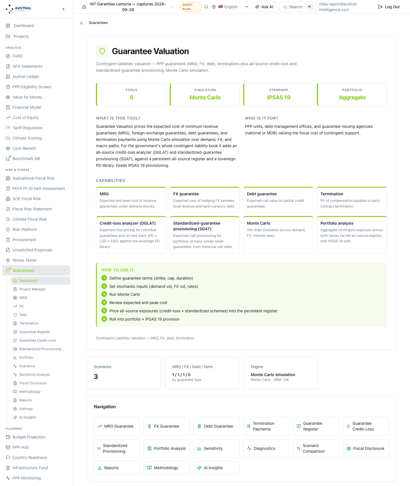
Platform module that runs the method: Guarantees (/guarantees) — "Guarantee and Contingent Liability Valuation", and specifically its all‑sources half: the guarantee credit loss analyzer (guarantees/credit-loss), the standardized guarantee provision (guarantees/standardized-guarantee), the sovereign PD library and the IPSAS 19 disclosure note (guarantees/fiscal-disclosure) — with destinations in the Fiscal Risk Statement (/frs, manual M9), the Austral Ledger's IPSAS 19 classification (/ipsas) and state‑owned enterprise fiscal risk (/soe, manual M6)
Languages: English (this edition) and Spanish · HTML and PDF at austral‑intelligence.com/manuals
This manual explains how to answer four questions about a State's book of guarantees: how much it has guaranteed outside the public‑private partnership contract, to whom, with what probability of being called on it, and how much of that has to go on the balance sheet this year. It presents the valuation of guarantees and contingent liabilities as a self‑contained eleven‑step method running from the perimeter to the report, built on two corrections it states as its thesis: the face value of a guarantee is not its cost, and the expected cost of a guarantee is not, on its own, its provision. It splits the universe by the partition that decides everything — the one‑off guarantee, assessed one by one and not recognized unless its call is shown to be probable, against the standardized guarantee scheme, assessed on its own history of calls and recognized as a liability from day one — and it credits each rule to its source: the two guarantee tools of the IMF's fiscal risk toolkit, the Government Finance Statistics Manual 2014 with the System of National Accounts 2008, IPSAS 19 and IPSAS 41 with IPSAS 28, the credit risk literature and five national practices. Where those sources disagree the manual takes a declared position rather than inventing a consensus, and the central case is one it does not soften: three rulebooks in force do not give the same answer about the same guarantee, and the manual sets out both accounting standards, applies IPSAS 19 and publishes the figure the other would put on the balance sheet. Its most consequential result is that the probability compared with the standard's threshold must be the probability of some call over the life of the guarantee and not the annual one — a correction that, in the worked example, moves the contingent liability provision by almost five times and brings onto the balance sheet precisely the most expensive guarantee in the book. It walks the eleven steps through a complete twelve‑row register of the fictitious Republic of Lemuria, with every figure shown; shows how the method runs on the Austral platform, screen by screen, with what it does not yet do declared as such; and explains why this particular method breaks in a spreadsheet. It is written for debt offices, ministries of finance, government accountants, statistics offices, guarantee fund managers, parliaments and auditors.
Austral Intelligence (2026). Government Guarantees and Contingent Liabilities from All Sources. Manual M7, Austral Manual Series, version 1.0, September 2026. https://austral-intelligence.com/manuals/government-guarantees/
Every figure in the worked example (section 4) and in the screenshots (section 5) is generic: it belongs to the fictitious Republic of Lemuria's twelve‑row demonstration register — eight one‑off guarantees and four standardized schemes — shipped as a demonstration pack in the platform and calibrated so the method can be followed from start to finish. None of it comes from a client or a real programme, and none of it should be used as a reference for the exposure, the cost or the provision of any actual guarantee book. GDP for the worked example is a declared assumption (60,000, in millions of Lemuria's currency), and every "% of GDP" figure in the manual carries it alongside; none of the method's decisions depend on it. The discount rate (6%), the default correlation (0.30), the stress multiplier (×2) and the "remote" cut (5% on the lifetime probability) are declared assumptions or Austral conventions, not thresholds of any source, and the manual says so where each one applies — the standard exempts the remote from disclosure without putting a number on it. The portfolio tail layer uses 50,000 draws with a fixed seed, published so that a reviewer can reproduce the figure; the analytical figures reproduce to the cent and the simulated ones are stable but not exact, and section 4's annex says which are which. The methodologies cited are credited to their authors; the only product name in the manual is Austral.
This is the first English edition of Manual M7, translated from the Spanish version 1.0 (25 September 2026). Every figure, table and citation is carried over unchanged; where the two editions differ, including after a future correction to either one, the Spanish edition is the reference. Two places were adapted rather than translated, and both are declared where they occur: the cross‑edition note in §2.3, which in Spanish maps the IPSASB's official Spanish acronym and paragraph prefixes onto the English ones and here keeps only what a reader checking one edition against the other still needs; and the citation status of the OECD Arrangement in §2.6 and reference 19, where this edition verified the status, the Participants and the scope in English and could not verify the literal English wording of articles 20 and 21, and says why.
A ministry of finance signs guarantees. A guarantee on the railway company's debt, a guarantee on a regional government's bond, a fund backing loans to small firms, a State guarantee on student credit, an agricultural insurance scheme run by another ministry. None of those obligations is in this year's budget, almost none is in the public debt the country publishes, and in most ministries none of them is valued: the guarantee book is a list of authorized amounts that someone keeps in a spreadsheet, split between the debt office, the manager of each fund and a budget annex. This manual answers four questions about that book: how much has the State guaranteed outside the public‑private partnership contract, to whom, with what probability of being called on it, and how much of that has to go on the balance sheet this year.
The thesis fits in two sentences, and they are worth stating before the method. The face value of a guarantee is not its cost, and the expected cost of a guarantee is not, on its own, its provision. The first is a measurement error: the guaranteed amount is what the State would pay if everything failed and nothing was recovered, and most guarantees are never called. The second is a rulebook error: an expected loss is a measure of risk, and whether it is recognized on the balance sheet is decided by an accounting rulebook that treats the individual guarantee and the mass scheme differently. A register that confuses the first reports a figure five to seven times larger than the one that has to be budgeted; a register that confuses the second leaves off the balance sheet, precisely, the most expensive guarantee in the book. Those two corrections are the structure of this manual.
The question is: how much have I guaranteed, to whom, with what probability of being called on it, and how much of that goes on the balance sheet this year? The product is a valued register of the conditional obligations the State has written, whoever the guaranteed debtor is: each guarantee with its exposure, its probability, its expected cost and its accounting and statistical treatment; and the whole book with its tail, its concentration and its position against the ceiling.
From that follows, with the same clarity, what it does not answer.
What this register is not
- It is not an appraisal of the project or of the policy. It does not say whether the guarantee was a good idea, whether the project that received it is worth what it costs, or whether the beneficiary deserved it. It prices an obligation that is already written. To decide whether granting it is worthwhile — and at what price — the manual offers Step 8, which is a piece of design, not a judgement on the programme.
- It is not a diagnosis of the guaranteed debtor. If the debtor is a state‑owned enterprise, what says whether it is well run, whether it is solvent and whether it should sit inside government is M6. This manual takes that reading as an input to the probability and does not produce it.
- It is not the register of firm and contingent commitments of the public‑private partnership contract. The minimum revenue guarantee, the exchange‑rate guarantee and the compensation for early termination are born of a contract, have a formula and are valued as options on a state variable. That is M2, and the border is written in one line (§2.5).
- It is not a debt sustainability analysis. It does not say whether the country can borrow more. It says how much conditional debt it has written and what it is worth.
- It is not the fiscal risk statement. The register enters that statement as two families with four figures each; building the statement, consolidating it with the other sources of risk and setting the aggregate ceiling is M9.
The five manuals of the first wave are about the public‑private partnership contract; the sixth is about the state‑owned enterprise. This one is about the instrument, and the difference is not of sector but of the nature of the object.
A public‑private partnership contract has a schedule and a financial model. The availability payment is written down, the minimum revenue guarantee has a formula, the termination compensation has a calculation base. The analytical work consists of reading the clauses and simulating the variables they depend on.
A state‑owned enterprise has a balance sheet. There is no clause saying how much the State will pay next year; there are financial statements, an ownership relationship and three channels through which the risk reaches the budget.
A guarantee has neither. It has four things, and nothing more: an issuer — the State — a beneficiary, a covered obligation and a trigger. There is no flow to project, because until the trigger fires the guarantee costs nothing; and when it fires it costs, all at once, a fraction of the covered amount. That is its entire economics, and from it comes the result that makes this manual possible: the origin of the guaranteed debtor changes who fails, not how it is valued. A guarantee to a state‑owned enterprise, to a regional government, to a development bank, to an agricultural cooperative or to a student all come through the same door and are valued under the same law. That is what allows a ministry to have one guarantee register instead of five disconnected books, each in the office that issued its own guarantee.
There is a second difference, less comfortable, and it is about governance. In a contract, the perimeter is given: the contract exists or it does not. In a guarantee book, the perimeter is the problem: guarantees are issued by several entities, written into different laws, kept in different files, and nobody has the complete list. The commonest defect in this discipline is not a calculation error but a guarantee that is not in the register because whoever signed it did not know there was a register. Step 0 and Step 9 exist for that.
Before any formula the universe has to be split in two, and the split is not about size: it is about the method of valuation and the accounting treatment.
A one‑off guarantee is individually material and is assessed one by one: it has a named debtor, a balance, a term and a probability that someone has to justify. A standardized guarantee scheme is a population of small and similar guarantees — loans to small firms, student loans, agricultural insurance, mortgage guarantees for social housing — assessed on its own history of calls, because assessing each one would be impossible and, besides, unnecessary: the law of large numbers makes the annual flow an estimable figure.
The accounting consequence is asymmetric, and almost no register writes it down: the standardized scheme generates a recognized liability; the one‑off guarantee does not, unless its call is shown to be probable. A scheme is called every year — that is its point — so its expected flow is a measurable present obligation and goes on the balance sheet without further ado. A one‑off guarantee has to pass a probability test first, and half the value of this manual lies in applying that test on the right base (§2.3 and Step 7).
This is not a project instrument: it is a calendar instrument, and it is run at three moments.
On granting. Before signing: the authorization, the position against the ceiling, the break‑even price, the fee that will be charged — or the explicit decision not to charge it, which is a subsidy — and the entry in the central register. It is the only moment at which the policy can still be changed.
Every year. With the close of the financial year: revaluation of every row, review of each scheme's call rate, the provision, the disclosure note and the report to the fiscal risk statement. Along with M2 and M6, this is one of the three manuals in the series that is run every year and not once per transaction.
On an event, outside the calendar: a guarantee called, an arrear by the guaranteed debtor, a deterioration in its rating, the renewal or the enlargement of a scheme. The rule in Step 5 is explicit: a guarantee that has already been called once stops being a row in the register and becomes a case, with its own note and its probability revised by hand.
The annual product feeds three calendars that are not its own: accounting (the provision to the balance sheet, the contingency to the note), statistics (what is a liability and what is a memorandum item) and the budget with the fiscal risk statement that accompanies it. Step 10 settles which figure goes to which and how they must reconcile with each other.
Seven readers, seven uses of the same register, and no two of them read the same column.
Two warnings about that division of labour. The first: whoever operates the tool does not decide the perimeter. Whether a guarantee is or is not in the register, and whether a scheme is or is not standardized for measurement purposes, has accounting and statistical consequences that belong to government accounting and to the statistics office; the analyst applies the test, documents it and takes the result to whoever has to decide it. The second: a published probability has consequences. Saying that a state‑owned enterprise's debt has a 95% probability of being honoured by the State over the next ten years affects that enterprise's cost of funds. Step 9 takes that up as a disclosure rule — aggregate portfolio and methodology always; debtor‑by‑debtor detail with the debtor forewarned — and not as an excuse for not publishing.
For each guarantee and for the whole register, the method produces five figures and a list. The six go together: published on its own, any of the first five is misread.
And the sixth, which almost no register writes down: what was not valued, and why. Implicit guarantees, which are named and not costed; guarantees issued by entities that do not pass through the central register; schemes administered outside the finance ministry; financial‑sector guarantees that another law regulates. It is the list that makes the other five auditable.
The first three measure different things in different units, and the manual never adds them up. One is a stock that could be lost in full, another is the same stock net of recovery, the third is an expected flow. Adding two of them produces a number that means nothing and that, invariably, someone quotes.
These are the two errors that order the manual, and they deserve their own heading because they are the thesis.
The first, from above. A register that publishes only the guaranteed amount reports a figure that, in the example in §4, is 11,010 against 1,733.7 of expected cost for the whole register in present value: more than six times. To the minister who has to budget this year's payouts it says nothing. But the obvious correction — publishing only the expected cost — hides the other half of the problem: in that same example the 95% CVaR of the one‑off guarantee portfolio is 2,090.4 against a mean of 1,454.1, half again as much, and those 636 of difference have to be somewhere, because it is the tail that breaks a budget, not the mean. Hence the rule that Step 4 turns into a decision table: the three bases are always published together, and none of them replaces the others. A register that publishes only one of the three is always hiding something.
The second, from inside. An expected loss is not automatically a provision: the standard decides, and the standard decides differently for the one‑off guarantee and for the scheme. A register that provisions everything overstates the recognized liability. But the expensive error is the opposite one, and it is an error of base: applying the probability test to the annual rate instead of to the probability that the guarantee is called at some point in its life. A ten‑year guarantee with an annual probability of 26% "does not reach 50%" and stays off the balance sheet, when the probability that it is called at some point in those ten years is 95.1%. In the example in §4 the difference between the two readings is between 279.6 and 1,334.1 of contingent liability provision — almost five times — and what enters the balance sheet once it is corrected is, exactly, the most expensive guarantee in the book. The conversion that avoids that error fits in one cell: P = 1 − (1 − h)^n. Step 3 prints it every time the two probabilities appear together.
The two corrections have the same root, and it is the one the house has been arguing for some time: a guarantee is valued on the distribution and not on the mean path, because on the mean path almost any guarantee is worth zero (Austral, Foundations for Deciding When to Use a Third‑Party Guarantee). That the liability goes unvalued is not a technical accident (Austral, The Useful Silence), and the distance between what the rulebook obliges one to recognize and the tail the sovereign actually carries is measurable (Austral, The Recognition Rule). This manual measures it.
Three things, in the order of the series.
A self‑contained method. Section 3 develops eleven steps — from the perimeter to the report — with what goes in, what comes out and what the decision rule is at each one, and closes with the reviewer's checklist. It is written to be applied with a spreadsheet and a folder of evidence, without depending on any particular tool. Section 2 credits each rule to its source by section or paragraph — the two guarantee tools of the International Monetary Fund's fiscal risk toolkit, the Government Finance Statistics Manual 2014 with the System of National Accounts 2008, IPSAS 19 and IPSAS 41 with IPSAS 28, the credit risk literature and five national practices — and says where the sources do not agree: in this manual there are three rulebooks in force that do not give the same answer about the same guarantee, and resolving that without softening it is what makes it useful.
A reproducible example. Section 4 runs the method over a complete twelve‑row register — eight one‑off guarantees and four schemes — with one guarantee almost certain to be called, two that the annual reading was hiding, three that the term takes out of the remote category, one scheme that costs more than all the others put together and charges nothing, and one that is self‑financing on average and stops being so under stress. Never a client's data.
The tool that runs it, and that the client keeps. Section 5 shows the module screen by screen, with what it records, what it exports and what it does not yet do, declared as such. Section 6 is honest about the spreadsheet argument: the tools this method reimplements are spreadsheets, and good ones; what the manual disputes is not that spreadsheet but what happens to it when it stops being a diagnostic instrument and becomes the annual register of a hundred guarantees and eight schemes with a reporting chain behind it. Section 7 gathers the references with their verification status.
A reader who only needs to know whether a guarantee book arriving for signature is well made can go straight to the reviewer's checklist at the close of section 3. A reader who wants the logic in one page, to the summary in 3.11.
Every rule in §3's method comes from a tool a ministry of finance applies, from a statistical or accounting rulebook that requires it, or from a national practice that has tested it. This section says where each one comes from, by section or paragraph, so the reviewer can dispute the rule in its source and not in the manual. The sources fall into four bodies. One primary source of method: the International Monetary Fund's fiscal risk toolkit, from which this manual uses two pieces — the tool for one‑off guarantees and loans and the tool for standardized guarantee schemes — which give the split of the universe into two families and the formulas for each. Three rulebooks that do not say the same thing about the same guarantee: the Government Finance Statistics Manual 2014 (GFSM 2014) with the System of National Accounts 2008 (SNA 2008), which say what counts as a liability of the State; IPSAS 19, which says when a conditional obligation is recognized on the balance sheet; and IPSAS 41, which says that some of those same guarantees do not go through that test because they are financial instruments. One source from the finance literature: the expected credit loss identity, the reading of a guarantee as an option and the one‑factor portfolio model, which give the probability, the severity and the tail. And five national practices. Table 2.9 links each step of §3 to its source and to the §5 screen that runs it.
A reading warning, on the three points where the sources do not agree and the manual adopts a declared position, not an invented consensus. (i) Statistics leave the one‑off guarantee off the balance sheet — a memorandum item — and put the standardized scheme on it; accounting does not make that split in the same way. (ii) IPSAS 19 recognizes nothing until the call is probable; IPSAS 41 measures a guarantee on a third party's debt by expected credit loss, with no prior probability test, and IPSAS 19's scope expressly excludes what IPSAS 41 covers. The manual sets out both standards, applies IPSAS 19 — which is what the §5 tool runs — and flags every place where IPSAS 41 would require something else, with the figure for the effect in §4. (iii) The implicit guarantee is valued in none of the three books and this manual does not value it either: it names it, argues it and leaves it without a figure, saying why (§1.6 and Step 10).
And a warning about method. This manual rests on two documented Fund tools other than PFRAM, and the §5 module is a reimplementation of their published method, not a copy of their files. That is why §2.1 credits each tool by name and source, says what it takes and where the reimplementation departs, and uses neither tool's name as a section name or a product name. The only product name in this manual is Austral.
And a warning about terminology. The accounting terms in this manual are the issuer's own English terms, not market usage and not a house coinage: provision, contingent liability, legal obligation and constructive obligation, obligating event, probable, remote, best estimate, expected value; and on the financial instruments side, financial guarantee contract, loss allowance, expected credit losses, cash shortfalls and credit risk. The switch between the two measurement horizons is written as the standard writes it: credit risk has increased significantly since initial recognition. One point of usage that English keeps apart and the Spanish edition of this manual has to signpost: constructive obligation — the IPSAS term for an obligation arising from an entity’s established pattern of practice rather than from law — is not the implicit guarantee of the perimeter sections, which is the expectation of rescue without a clause. In English the two are different words and no confusion arises; the reader moving between the two editions should know that the Spanish renders both with the same adjective.
And the vocabulary that has no official form, declared here as the house's own because the manual uses it in every section. "Probability test": IPSAS 19 names no test — ¶22 states three simultaneous conditions and ¶31 defines "probable" — just as M8 declares its "control test". "Expected loss", "severity", "face value" and "maximum exposure" come from the two Fund tools and from the credit literature in §2.4, not from the IPSASB: they must not be confused with the expected credit loss of IPSAS 41, which is a different measure under a different rule — §2.3.2 explains where they part company — nor with the expected value of IPSAS 19 ¶47, which is official form and is used in that sense. "One‑off guarantee" and "standardized guarantee scheme" are from GFSM 2014 and SNA 2008; they are official, but statistical and not accounting, and §2.2 credits them there.
The Fiscal Risk Toolkit of the Fund's Fiscal Affairs Department is a family of spreadsheet tools for fiscal risk analysis; its pieces, in the current diagram, are the high‑level fiscal risk assessment instrument, the state‑owned enterprise health check and stress test (the subject of M6), the PPP fiscal risk model (PFRAM, the subject of M2), the public sector balance sheet assessment, the fiscal stress test, the quantitative climate risk tool, and the two guarantee tools this manual uses. The composition of that family, with its diagram, is described in the evaluation that the Fund's own Independent Evaluation Office published on 16 December 2025 (p. 11: figure 1 and ¶21–22), which is the most recent published source on the toolkit and the one this manual uses to credit it.
Three things are worth retaining from that page. The first, about attribution: of all the pieces in the toolkit, the only one the evaluator declares to have been built jointly with the World Bank is the PPP fiscal risk model; the two guarantee tools are the Fund's, and whoever cites them as joint work is attributing them wrongly. The second: neither of the two is a complete guarantee management system; they are two pieces answering two different questions about two different populations, and that split is what orders the whole manual. The third is that the toolkit is not a fixed list: the December 2025 diagram is not the one in the 2021 and 2023 user guides — the pandemic stress test goes out, the climate tool comes in, and the acronym of the one‑off guarantee tool changes — so citing the toolkit obliges one to date the photograph. M9 draws from this a rule of method that this manual shares: one registers the family, not the instrument.
The tool for one‑off guarantees and loans is published today under the acronym DGLAT, and that is the acronym this manual uses for it. Its long name, by contrast, is not a single one, and the manual does not choose: on that same page 11 of the evaluation, figure 1 — which is the Fund's own diagram — expands it as Debt Guarantee and Loan Assessment Tool and ¶22 as Discrete Guarantees and Loans Assessment Tool. Both expansions are the publisher's, they are in the same document, and neither is corrected by the other; presenting one as the right one would be a false citation. The acronym is the only stable thing, and it is what is used. (The variant DGAT, without the L for "Loans", is the one from the toolkit's earlier diagram — that of the user guides of November 2021 and January 2023, where the tool was expanded as "Discrete Guarantee and Loan Assessment Tool". It is recorded here once, because it explains why the acronym appears in two forms in the literature and on the screens.) The tool assesses "fiscal risks from one‑off debt guarantees and loans to non‑financial SOEs" and, in the evaluator's words, "estimates expected fiscal costs and maximum exposures on entity‑specific loans and guarantees". From it the manual takes four things, in the order in which §3 runs them. First, the object: the individually material guarantee, assessed one by one, together with the government's direct loan to the same debtor — the tool handles both on the same board, and §3 Step 0.3 inherits that decision with a warning of its own that the source does not write (§2.4). Second, the valuation chain: the tool "uses a credit scoring approach to assign a risk rating to each entity based on their financial health and business risk characteristics" and then "translates borrower risk ratings into probabilities of distress"; that is, the probability is not invented, it is derived from a documented diagnosis of the debtor. Third, the two output figures, which the source names separately and never adds together: "calculates maximum fiscal exposure and estimates of expected losses based on assumptions". And fourth, what the result is for: "can help inform ex‑ante decisions on whether to extend guarantees, setting risk‑based guarantee fees, risk mitigation, budget provisions and ongoing risk monitoring" — the five decisions of §1.4, including the risk‑based fee that is Step 8 of this manual.
The source also grades its own data requirements in three levels, and that grading is exactly the one §3 uses to tell the reader how far they can get with what they have. Basic version — risk rating on the stocks: the debtor's financial statements, business risk information and stocks of loans and guarantees. Full version — expected loss: the above plus macro‑fiscal and market data, the financial characteristics of each loan and guarantee including its amortization profile, the probability of credit events and the expected loss given the event, instrument by instrument. Extension — stress test: a shock scenario for output, exchange rate or interest rates, and the sensitivities of the probabilities to those macro variables. Note the order: the term and the amortization profile enter at the level where expected loss is calculated, not at the inventory level. A register that publishes an expected loss without declaring the term of each guarantee is reporting a full‑version figure with basic‑version data, and §3 Step 3 treats that as an error of base, not as a rounding.
The tool for standardized guarantee schemes — Standardized Guarantees Assessment Tool, SGAT; here there is no variant to declare: the name and the acronym are the same in the evaluation and in the presentation material — is the complementary one. The evaluator sums it up as the one that "values scheme‑level portfolios under baseline and stress cases to inform pricing, provisioning, and disclosure", which are the three decisions of Steps 3, 8 and 7 of §3. And the department itself presents the two as a pair: "both estimate the fiscal costs and risks from guarantees and loans", with the first focused on the one‑off guarantee and this one on schemes. It quantifies "the fiscal costs and risks from standardized guarantees or loan schemes using baseline and stress scenarios"; the method is a cash‑flow‑based portfolio analysis that models the aggregate behaviour of the debtors, not a sum of individual assessments; its declared use case is credit schemes for small and medium‑sized enterprises; and it is built to accommodate the features that distinguish one scheme from another: "risk coverage, loss sharing, pricing, collateralization". What the manual takes from here is the rule of partition and the unit of analysis: in a scheme one does not estimate the probability that a particular debtor fails — that is impossible and also unnecessary — one estimates how many of a batch of similar loans will fail, and the estimate rests on the scheme's own history. Step 5 and half of Step 7 come from there.
Where Austral's implementation departs from the source, and why. The §5 module is not a line‑by‑line translation of either tool; it is a reimplementation of their method, and the differences are declared here because presenting them as the Fund's would be a false citation.
(On the user guide for these two tools: it does not exist. As at 24 September 2026, the publisher's pages corresponding to the user guide for the one‑off guarantee and loan tool and for the standardized scheme tool announce the document as forthcoming. There is therefore no title, authorship, year or section numbering to fix — unlike the two state‑owned enterprise tools of the same toolkit, whose user guides are published. The check was made twice and separately on the same day. §2.1 is then credited with what is published and is the publisher's own: the evaluation by the Fund's Independent Evaluation Office (2025, p. 11), which describes the toolkit and names and summarizes the two tools, and the two presentations by the Fiscal Affairs Department (Rentería 2023 and Frank 2025), which give the scope, the valuation chain, the outputs and the three levels of data requirements. When the publisher releases the guides this section will have to be read again: if they describe the method differently, §2.1 gets rewritten.)
This is the most consequential part of §2, because half of Step 7 comes out of it and because it explains why two guarantees that look the same to a reader turn up in two different places in the public accounts. The two sources — GFSM 2014 and SNA 2008 — say the same thing here, and it is worth making the most of it: it is the only one of the three rulebooks where there is no conflict to declare.
Three classes of guarantee, not one. SNA 2008 says so in its ¶17.209 — "three classes of guarantees are recognized" — and develops them in ¶17.210 to ¶17.212: those provided by means of a financial derivative (a credit default swap, which is traded on the market and is not tied to an individual loan); standardized guarantee schemes; and one‑off guarantees. GFSM 2014 takes up the same partition and adds the balance sheet consequence in a sentence worth quoting in full (¶7.253): "not all guarantees are contingent liabilities; as discussed earlier in this chapter, guarantees in the form of financial derivatives and provisions for calls under standardized guarantee schemes are liabilities on the balance sheet. On the other hand, one‑off guarantees are contingent liabilities."
The line that separates the scheme from the one‑off guarantee is not size. GFSM 2014 draws it with two criteria (¶A4.71), and SNA 2008 with the same two (¶17.213): the scheme "is characterized by frequently repeated transactions with similar features and pooling of risks", and its guarantor "is able to estimate the average loss from the available statistics using probability‑weighted concepts". The one‑off guarantee is the opposite, and for the same reason: "one‑off guarantees are individual, and guarantors are not able to make a reliable estimate of the risk of calls" (GFSM 2014 ¶7.256 and ¶A4.71). The logic is that of non‑life insurance and both sources say so in those words: one cannot know which debtor fails, but one can know how many of a batch of similar debts will, and "it is standard practice to estimate how many out of a batch of similar debts will default" (¶A4.71). The examples the two sources give are the same and are useful for Step 1: export credit guarantees, deposit insurance and student loan guarantees (GFSM 2014 ¶7.202 and ¶A4.72; SNA 2008 ¶17.211).
The asymmetry, which is the thing that has to be written down. The standardized scheme creates a liability: "operators of standardized guarantee schemes incur liabilities equal to the present value of the expected calls under outstanding guarantees, net of any recoveries the guarantor expects to receive from the defaulting borrowers, a similar approach as for nonlife insurance. This liability is called provisions for calls under standardized guarantees" (GFSM 2014 ¶7.201). Three points of precision in that sentence, which §3 Step 3.2 turns into calculation rules: the liability is at present value; it is of the expected calls on the guarantees outstanding, not of this year's; and it is net of expected recoveries. The one‑off guarantee, by contrast, is not recorded: "in most cases, a one‑off guarantee is considered a contingent liability of the guarantor. Liabilities under one‑off guarantees continue to be attributed to the debtor, not the guarantor, unless and until the guarantee is called" (¶7.257). SNA 2008 says the same in its ¶17.212, and adds the treatment of the fee and of the call: the fee charged is payment for a service, and the call is a capital transfer from the guarantor to the beneficiary — or a financial transaction, if the guarantor obtains an effective claim on the guaranteed party.
The two exceptions, which are the ones a ministry meets in practice. (a) The one‑off guarantee granted to an enterprise in financial difficulty and with a very high probability of being called "is treated as if the guarantee is called at inception" (GFSM 2014 ¶7.258; SNA 2008 ¶17.212): its activation is treated as debt assumption and the liability moves onto the guarantor's balance sheet. GFSM's note 75 adds the practical guidance that Eurostat applies and that is worth having written down, because it is the operational criterion that closes the "from when is it debt?" argument: if the government, as guarantor, pays on the same guaranteed debt in three consecutive years and the situation is expected to continue, the debt is considered assumed, normally in full — or in the proportion the government is expected to pay, if there is evidence for it. (b) The scheme with no fee, or with fees far below the calls and administrative costs, requires the unit operating it to be treated as a non‑market producer inside general government (GFSM 2014 ¶A4.72; SNA 2008 ¶17.223), with the consequence that neither source disguises: if the government recognizes the likelihood of financing part of the calls to the point of including a provision in its accounts, a transfer is recorded for that amount and a liability of the same amount. It is the border with M6 and it goes in writing: who operates the scheme decides where the liability appears, not whether it exists.
What gets published of what is not recorded. GFSM 2014 recommends that publicly guaranteed debt (6M61) be shown at nominal value as a memorandum item to the balance sheet and, if significant, also other one‑off guarantees (6M62) and the remaining explicit contingent liabilities (6M63) (¶7.254–7.255). And it acknowledges on the same page, in its note 74, the limitation this manual turns into its opening thesis: that approach "offers no information on the likelihood of the contingency occurring and it may overstate the possible risk. For loan and other debt instrument guarantees, the maximum potential loss is likely to be less than their nominal value, because not all debts will default." The rulebook itself says that face value is not the cost, and asks for metadata on the valuation method used. Read that way, this manual is an answer to that footnote.
And what statistics expressly leave out. GFSM 2014 distinguishes explicit and implicit contingencies (¶7.252) and lists among the latter, in so many words, "ensuring the solvency of the banking sector, covering the obligations of subnational governments (state and local governments) or the central bank in the event of a default, assuming unguaranteed debt of public sector units, and potential spending for natural disaster relief". The unguaranteed debt of a state‑owned enterprise is, in the rulebook itself, an implicit contingent liability of the State. This manual does not value it — by the rule in §1.6 — but it does register it, and refers out to M6, which is where the debtor is diagnosed.
A government accountant reading §2.2 will ask the question on the first page: if statistics leave the one‑off guarantee off the balance sheet, does accounting do the same? The answer is that it depends which of two standards applies, and both are in force. This section sets out both without softening them.
A note on terminology and editions, before going in. The literal quotations in this section are taken from the issuer's pronouncements in English, 2025 edition — amendments issued through 31 January 2025 — which is the edition that fixes the numbering used here; the individual standards, IPSAS 19, IPSAS 28 and IPSAS 41, were read directly in the issuer's published English text for this edition. The terms are therefore the issuer's own and need no equivalence: provision, contingent liability, legal obligation and constructive obligation, obligating event, probable, remote, best estimate, expected value; and on the financial instruments side, financial guarantee contract, loss allowance, lifetime expected credit losses, 12-month expected credit losses, cash shortfalls and credit risk.
Three warnings a reader needs in order to check any citation in this section against the other edition of this manual.
Recognition. IPSAS 19 ¶22 requires three simultaneous conditions for a provision to be recognized: a present obligation (legal or constructive) as a result of a past event; that it be probable that an outflow of resources will be required to settle it; and that a reliable estimate can be made of the amount. "If these conditions are not met, no provision shall be recognized."
What "probable" means, with a number. ¶31 leaves no margin: "for the purpose of this Standard, an outflow of resources or other event is regarded as probable if the event is more likely than not to occur, that is, the probability that the event will occur is greater than the probability that it will not." It is the 0.5 threshold that §3 Step 7 applies, and it is the only number the standard puts down. ¶32 adds the rule that decides the case of the standardized scheme: where there are a number of similar obligations, the probability that an outflow will be required is determined by considering the class of obligations as a whole; although the likelihood of outflow for any one item may be small, "it may well be probable that some outflow of resources will be needed to settle the class of obligations as a whole", and then the provision is recognized. It is the same asymmetry as in §2.2, written now in accounting language and for another reason: not because statistics require it, but because the probability test applies to the class and not to the individual.
What happens when it is not recognized. ¶35 is blunt: "an entity shall not recognize a contingent liability." And ¶36 says what is done instead: "a contingent liability is disclosed, as required by paragraph 100, unless the possibility of an outflow of resources embodying economic benefits or service potential is remote." From there come the two exits of Step 7 — recognized provision or disclosed contingent liability — and the third, the remote one, which requires no disclosure. Note the exact assignment of paragraphs, because it is easy to get wrong and this manual corrects it against its own working index: ¶35 is the prohibition on recognizing; ¶36 and ¶100 are the disclosure and the exemption for the remote case. The standard puts no number on "remote"; the cut the module applies is an Austral convention and is declared as such (§5.2).
How what is recognized gets measured. ¶44 sets the general rule: "the amount recognized as a provision shall be the best estimate of the expenditure required to settle the present obligation at the reporting date." ¶47 says how that best estimate is arrived at when the obligation is a population: "where the provision being measured involves a large population of items, the obligation is estimated by weighting all possible outcomes by their associated probabilities. The name for this statistical method of estimation is 'expected value'." And ¶48 says what is done with a single obligation: "the individual most likely outcome may be the best estimate of the liability", with the caveat that the other outcomes be considered. A standardized scheme is measured, then, at expected value, which is exactly what §3 Step 3.2 computes; a single one‑off guarantee is measured at the most likely outcome, with ¶48's own qualification. And ¶53 closes the arithmetic: "where the effect of the time value of money is material, the amount of a provision shall be the present value of the expenditures expected to be required to settle the obligation", at the rate of ¶56 — "a pre‑tax rate (or rates) that reflect(s) current market assessments of the time value of money and the risks specific to the liability", which "shall not reflect risks for which future cash flow estimates have been adjusted". That last sentence is the one that stops the same risk being discounted twice, and §3 Step 3 applies it literally.
The consequence for the base of the probability, which is the most expensive decision in the manual. The provision is measured at the expected value of the obligation, not at one year of it, and is discounted to present value. If the measurement is lifetime, the ¶22 test has to be on the same base: the probability compared with 0.5 is that of some call over the life of the guarantee, not the annual one. It is the rule M2 set for the series and that this manual inherits unchanged, and its effect is not marginal: in the example in §4, applying the test to the annual probability leaves precisely the most expensive guarantee in the register off the balance sheet, and the conversion P = 1 − (1 − h)^n is the only thing separating the two readings. §4.7 publishes both and the difference.
Scope, which is where the conflict starts. IPSAS 19 applies to provisions, contingent liabilities and contingent assets except — ¶1(e) — those "covered by another IPSAS"; and ¶4 names the exception that matters here in so many words: "this Standard does not apply to financial instruments (including guarantees) that are within the scope of IPSAS 41, Financial Instruments."
The definition. IPSAS 41 ¶9: "a financial guarantee contract is a contract that requires the issuer to make specified payments to reimburse the holder for a loss it incurs because a specified debtor fails to make payment when due in accordance with the original or modified terms of a debt instrument." Read it slowly, because it is the definition of the debt guarantee this manual values: a third party who does not pay a debt instrument, and an issuer who reimburses the holder for the loss.
And is a guarantee granted by law a "contract"? It is the immediate objection of any debt office, and the standard answers it. IPSAS 41 ¶AG131 bounds the scope — "only contractual financial guarantees (or guarantees that are in substance, contractual) are within the scope of this Standard" — and refers out to IPSAS 28. And IPSAS 28 ¶AG3 makes the precise distinction: "in assessing whether a guarantee is contractual or non‑contractual, an entity distinguishes the right to issue the guarantee and the actual issue of the guarantee. The right to issue the guarantee in terms of legislation or other authority is non‑contractual, while the actual issue of the guarantee should be assessed using the principles in paragraph AG20." ¶AG4 resolves it with two examples that read as though they were written for this manual: a guarantee issued directly to the financiers of a concession contract, and a guarantee that a national government grants by exercising its powers in legislation over a road authority's bond issue, with no identified counterparty, "implicitly issued in favor of the holders of a specific instrument". The standard's conclusion: "in both these scenarios, assuming that all the other features of a contract are met, the financial guarantee is contractual in nature." The power to guarantee is non‑contractual; the guarantee actually issued under that power is contractual. The guarantee authorized by a budget law and then written over a specific issue falls, on the letter of it, inside IPSAS 41.
And ¶AG20, to which ¶AG3 refers, is the one that sets the test: "an entity considers the substance rather than the legal form of an arrangement in determining whether it is a 'contract' for purposes of this Standard", and it gives three signs — that contracts "involve willing parties entering into an arrangement"; that "the terms of the contract create rights and obligations for the parties to the contract, and those rights and obligations need not result in equal performance by each party"; and that "the remedy for non‑performance is enforceable by law". That third point is the one a debt office must be able to evidence for its guarantee: it is not enough that the law authorizes it, there has to be a holder with an enforceable claim against the State.
How it is measured, and why that changes the result. Initial measurement at fair value (¶57). Subsequent measurement, ¶45(c): the issuer of a financial guarantee contract measures it "at the higher of: (i) the amount of the loss allowance determined in accordance with paragraphs 73–93; and (ii) the amount initially recognized (see paragraph 57) less, when appropriate, the cumulative amount of revenue recognized". There are two substantive differences from IPSAS 19 and it is worth separating them, because the manual treats them differently:
The consequence, written without softening it. The three bases §3 requires to be published are not three ways of saying the same thing: they are the three figures that three different rules ask for. The annual expected loss is the natural approximation to IPSAS 41's 12-month allowance for a newly granted guarantee with no deterioration; the lifetime expected loss in present value is IPSAS 19's measurement when the provision is recognized, and also IPSAS 41's when credit risk has increased significantly; and the face value is neither of the two, it is the ceiling of the authorization. A register that publishes a single figure will be, at best, answering one of the three questions and keeping quiet about the other two.
What this manual does with that, and what the tool does. The manual sets out both standards, applies IPSAS 19 — which is what the §5 platform runs, and what most ministries in the region apply today — and flags in Step 7 and in §4.7 every place where IPSAS 41 would require something else, with the figure for the effect. The platform implements no IPSAS 41 treatment today, and §5.6 declares that as a limit, not as a methodological decision. Leaving the question out would have been the comfortable option and the worst one: it is the first question a government accountant asks, and not having it answered takes authority away from the rest of the manual.
A note on the guarantee granted with no fee, which is the normal case in the public sector. IPSAS 41 ¶AG133 describes it without circumlocution: "in the public sector, guarantees are frequently provided by way of non‑exchange transactions, i.e., at no or nominal consideration. This type of guarantee is provided generally to further the entity's economic and social objectives." ¶AG134 asks that a market price for an equivalent guarantee be looked for first, and warns that the fact that the guarantee was given free "is not, of itself, conclusive evidence of the absence of an active market". ¶AG135 allows a valuation technique — and the example it gives is the credit spread between the coupon the bond would have paid without the guarantee and the one it pays with it. And ¶AG136 closes: if there is no reliable fair value measure by either route, the guarantee is measured at the amount of the loss allowance for expected credit losses. That chain — market price, failing that a valuation technique, failing that expected loss — is the same as Step 8's, and it is the reason this manual holds that measuring the price of a guarantee that is not charged for is not an academic luxury: it is what an accounting standard in force asks to be done first.
(Editions consulted: the text of IPSAS 19, IPSAS 28 and IPSAS 41 from the issuer's pronouncements, 2025 edition, incorporating amendments issued through 31 January 2025, read directly in the issuer's published English text; and, for the cross‑edition numbering check declared at the opening of this section, the issuer's official Spanish translation, 2022 edition. See §7.)
When the trigger of the guarantee is a debtor's default, valuation is a credit risk problem and the manual uses the standard identity of that field:
Expected loss = probability of default × severity × exposure,
EL = PD × LGD × EAD.
The identity comes from the internal ratings‑based framework of the Basel Committee on Banking Supervision, and it is cited as provenance, not as a standard applicable to the public sector. The distinction matters and goes in writing: no bank capital requirement binds a ministry of finance, and using Basel's vocabulary does not turn the Treasury into a bank. What is taken is the decomposition, because it separates three questions that a guarantee register confuses daily.
The probability (PD). Three legitimate provenances, in order of preference: the issuer's own history with that debtor or with that class of debtors; a credit rating translated into a probability by a published default study; or a documented judgement, with its basis written down. The manual publishes an indicative rating‑to‑annual‑probability table (§3 Step 3.1) with a warning that has to be repeated every time: those tables come from corporate default studies and are not calibrated for sovereigns or for state‑owned enterprises, whose default behaviour is different — a state‑owned enterprise rarely goes bankrupt; what it does is cost money. The table is an auditable starting point, not a standard.
The conversion the identity does not bring and the method requires. A rating table gives an annual hazard rate h. A guarantee is written for a term n. The probability that there is some call over the life of the guarantee is P = 1 − (1 − h)^n, and it is that one — not h — that enters the probability test of §2.3 and the measurement of the provision. The conversion is printed every time the two appear together, and its inverse h = 1 − (1 − P)^(1/n) too, because a register receives both forms depending on who fills in the record. The operating rule of §3 Step 3 is stricter than the arithmetic: with no term declared the method assumes none; the lifetime bases coincide with the annual one and the result says that the term was not declared. A term assumed by default is an invented figure with the appearance of a calculation.
Discounting. The expected flow is discounted at a declared rate, with the present value convention the series fixed in M2: present value is measured from the register's base year, and the base year is not discounted. It is what allows a present value from this manual to be added to one from M2 or M6 without anyone having to ask from which year each clock runs.
The severity (LGD). LGD = 1 − recovery rate, with the recovery declared and not assumed. Two warnings from Step 3. The first: a recovery of zero is not neutral, it is an assumption — and an expensive one, because it inflates expected loss as much as a 40% recovery reduces it; the engine does not assume it, it asks for it. The second: the recovery on a sovereign guarantee is not that of a secured bank loan, because the State that honours rarely enforces collateral and often ends up with a claim against a debtor that is its own. It is the case SNA 2008 ¶17.212 contemplates when it says the call may be recorded as a financial transaction if the guarantor obtains an effective claim.
The exposure (EAD). The guaranteed balance outstanding, not the amount originally authorized. It is the commonest error in registers kept on a spreadsheet, and it runs in two directions: a register that carries the original amount forward overstates the exposure of an amortizing guarantee, and one that omits accrued interest and indexation adjustments understates it. South African practice publishes the two figures separately precisely for this reason (§2.7).
The three figures that are never the same. Face value (EAD), maximum exposure on a full call (LGD × EAD) and expected cost (PD × LGD × EAD) are three different magnitudes, and the manual always publishes all three with their labels and never adds two of them together. The second is no longer the face value: it is what would be lost if everything were called and what was declared were recovered.
A case the identity does not cover and Step 0 separates: the direct loan. The two Fund tools handle government guarantees and loans on the same board, and the §5 module inherits that shared table. The manual keeps the conceptual separation even though the table is common, because an on‑lending in arrears is an impaired asset, not a contingent liability: its accounting treatment is the impairment of a receivable, not an IPSAS 19 provision, and adding them into a single "exposure" line is a category error that §3 Step 0.3 explicitly forbids. The expected loss arithmetic is the same; the place of the result in the statements is not.
The portfolio. Adding up the expected losses of the guarantees gives the portfolio mean and nothing else. For the tail, the manual uses the one‑factor Gaussian copula model — each debtor defaults when a latent variable, made up of a common systemic factor and an idiosyncratic term, crosses its threshold — the construction Vasicek published in 2002 as the limiting distribution of the value of a loan portfolio and which sits behind the asset correlation treatment of the Basel framework. From it come the VaR and the CVaR at 95%. What the model assumes, declared: a single correlation for the whole portfolio; binary defaults — everything or nothing is called, with no partial calls; and deterministic severity — recovery is not stressed along with the probability, when in a real crisis both move at once and in the same direction. And the pedagogical result that §4.5 measures with numbers: correlation does not move the mean and does move the tail. Raising it does not change what the portfolio costs on average; it changes how much has to be available for the year in which everything goes wrong. Two further warnings from Step 4: with few exposures the distribution has few atoms and the 95th percentile falls inside one of them, so the VaR becomes a step and stops being informative — the CVaR holds up better and is the one the manual recommends reading; and the correlation used is a declared convention, not an estimate, because a register of guarantees from all sources does not have the series of joint calls that estimating it would require.
Not every State guarantee is valued with PD × LGD × EAD. A minimum revenue guarantee, an exchange‑rate guarantee or a compensation for early termination has no debtor who defaults: it has a state variable — traffic, the exchange rate, a revenue stream — that crosses a threshold, and the object the State has written is an option. The manual's border rule, in one line:
This manual's method applies when the trigger is a debtor's default. When the trigger is the level of a variable, the method is M2's.
The theoretical reason is an old one and worth citing, because it is the bridge between the two manuals: Merton showed in 1977 that a guarantee on an entity's liabilities is isomorphic to a European put option written on its assets, and that its value therefore depends on volatility and not only on the expected level. From that follows the result that orders the two manuals in the series: valuing a guarantee on the mean path gives zero whenever the mean path does not cross the threshold, and that is precisely what a register does when it "values" the minimum revenue guarantee by applying the base case of the financial model. Irwin develops it for infrastructure in his chapter on valuing exposure and in the one on valuing the three risks, and it is the foundation of M2's simulation method.
This manual does not repeat that method: it names it, says when it applies and refers out. What it does inherit from M2, because it runs across the series, are three conventions — the conversion of annual probability into lifetime probability, the base year for present value and the recognition threshold on the lifetime probability — and the no‑duplication rule of Step 10: a minimum revenue guarantee in a concession contract is registered once and in M2, and appears in the all‑sources register only as a cross‑reference, never as a second line with a figure.
A guarantee is a financial service. It has a price, whether or not there is a fee that charges for it. The manual measures it with the break‑even premium: the level annual fee f whose present value equals the present value of the expected loss,
f · ä(T, r) = PV(expected loss), hencef = PV(expected loss) / ä(T, r), withä(T, r) = (1 − (1 + r)^(−T)) / r · (1 + r), andä(T, 0) = T.
The annuity is the one for payments at the beginning of each year — the first year's fee is charged when the guarantee is granted and is not discounted — which is the same clock as the base year with which §2.4 discounts the loss path. Both legs have to be on the same clock or the premium does not break even: using the annuity for end‑of‑year payments against a present value measured from the base year overstates the premium by the factor (1 + r), 6% at the rate in the §4 example. It is the standard par construction of credit protection — present value of the protection leg over the risky annuity — and it is the only one of the obvious candidates that actually breaks even: dividing the present value of the loss by the nominal number of years annualizes nothing, because it ignores the time value of the fee stream itself, and at long terms it collects about half the loss it is supposed to cover. Not annualizing at all is worse: it turns a whole‑life cost into an annual rate and exaggerates it by a factor of the order of the annuity.
Why it matters even when the State does not charge. The difference between the break‑even premium and the fee actually charged is the subsidy, and measuring it is the only way to say what a guarantee policy is worth. A scheme charging nothing is transferring exactly that amount to the beneficiary every year; a scheme charging above break‑even is taxing it. Neither is necessarily bad — a guarantee is a policy instrument and may well mean to subsidize — but both should be visible, and neither is if the register reports only face value.
And it is not merely good practice: an accounting standard in force asks for it. The chain in §2.3.2 — observable price of an equivalent guarantee; failing that, a valuation technique, and the example the standard gives is the credit spread with and without the guarantee; and only failing that, expected loss — is literally a pricing procedure applied to a guarantee granted free (IPSAS 41 ¶AG134–AG136). Irwin arrives at the same recommendation from fiscal policy in his chapters on charging fees and on using the market to value guarantees.
External order‑of‑magnitude benchmarks. To know whether a computed premium is reasonable it helps to look at published prices. The most useful is the OECD Arrangement on Officially Supported Export Credits, which governs eleven Participants and sets binding minimum premium rates for its members. Its Article 20 states the principle in two sentences that hold for any sovereign guarantee: Participants shall charge, in addition to interest, premia intended to cover the risk of non‑repayment, and those premia shall be risk‑based, shall converge between Participants and shall be adequate to cover long‑term operating costs and losses. Article 21 establishes that no Participant may apply a rate below the minimum premium rate, and lists the six factors that premium depends on: the country risk category, the duration of the risk (the horizon), the buyer risk category, the percentage of cover and the quality of the cover product, the country risk mitigation techniques applied and the credit enhancements applied. The premium is expressed "as a percentage of the principal amount of the credit as if the premium were collected in full at the date of first disbursement" — that is, a level premium expressed up front, the same convention as the formula above — and the calculation formula is in its Annex VI, with the qualitative description of the buyer risk categories in Annex IX.
Two warnings about that benchmark. The first is about scope: the Arrangement covers export credit with a repayment term of two years or more and is not a standard on domestic guarantees, so it serves as a reference for order of magnitude and for pricing structure, not as an applicable tariff. The second is about status: the text itself defines it as a non‑binding agreement among Participants — a "Gentlemen's Agreement" — that is not an Act of the Organisation. (The text consulted is the official one of January 2026; the English and French versions are both official, and the substance summarized here was read in the French version. [to be verified: the literal English wording of Articles 20 and 21. The publisher's legal‑instrument file carrying the English label reproduces the front matter in English but the body of the Arrangement in French only, and the publisher's document server returns a forbidden response for the paths that would hold the English body. That was not worked around, and the two Articles are therefore summarized here and not quoted.])*
([to be verified: the published tariffs of the multilateral credit insurers, which the working index proposed as a second benchmark. They were not opened for this edition and §2.6 does not depend on them.])
Five jurisdictions, chosen because they publish and because they differ from each other in something that matters. Structure, method and rules are cited; no client figures are used.
| Country | What it publishes, and under what rule | Frequency | Where it differs |
|---|---|---|---|
| United States | The subsidy cost of each federal guarantee and loan, in present value, budgeted when it is granted and not when it is called (Federal Credit Reform Act of 1990; the Office of Management and Budget's federal credit budgeting guidance) | Annual, with the budget | The benchmark case, and the only one of the five where the guarantee consumes budget appropriation in the year it is signed. The cost is "the estimated long‑term cost to the Government […] calculated on a net present value basis", discounted at the rate on Treasury securities of comparable maturity |
| Colombia | The valuations of contingent obligations of the contributing State entities, approved by the Directorate General of Public Credit, and the contributions to the Contingency Fund under a contribution plan (Law 448 of 1998; Decree 423 of 2001) | Annual, with periodic monitoring of how the risks evolve | The only one of the five with a funded provision and not merely an accounting one: the contribution is executed when it is transferred and is refunded only "when it is definitively established that the anticipated risks have not materialized" (cuando se verifique en forma definitiva la no realización de los riesgos previstos). Besides, each entity's valuation must be approved by the ministry, which may order the contributions raised or lowered |
| Chile | A dedicated annual report covering, in a single document, the two families of this manual: the State guarantee on state‑owned enterprise debt law by law, the higher education credit guarantee, the State deposit guarantee and the guarantee funds for small and medium‑sized enterprises, plus the pension system guarantees (Informe de Pasivos Contingentes, the Budget Directorate's contingent liabilities report) | Annual, under a legal mandate | The only one that declares its own recognition rule and says that it is more conservative than the international one: it acknowledges that the standard requires a probability greater than 50% and a reliable estimate, and expressly admits that its definition "is more conservative than the one mentioned and includes a wider range of obligations" (es más conservadora que la mencionada e incluye un rango más amplio de obligaciones). Also the one that best illustrates §2.2: the Treasury's guarantee to another entity of the public sector is treated as direct debt and falls outside the report; only guarantees granted to entities that are not part of the public sector come in |
| South Africa | The guaranteed amount and the exposure by entity, in the debt and contingent liabilities chapter of the Budget Review, with the full detail in the statistical annex | Annual, with the budget | The only one that publishes two distinct columns and explains why they are not the same. Also the only one that publishes concentration: the share of the two largest entities in total exposure |
| United Kingdom | Not a figure but a process: an approval framework requiring every new guarantee or indemnity to be scrutinized before it is granted, with a checklist and notification to Parliament, supported by a central Treasury capability (Contingent Liability Approval Framework, April 2023, within Managing Public Money) | Continuous, transaction by transaction | The only one that defines the contingent liability more broadly than the accounting standard — "commitments to use public funds if uncertain future events occur […] a wider definition than the accounting definition" — and the only one of the five with published guidance for implicit obligations (November 2025), which this manual does not value but does register |
Where they differ, along four axes. When the cost is recognized: the United States on granting, Colombia on contributing to the fund, Chile and South Africa on disclosing, the United Kingdom on approving. Whether it is funded: only Colombia, with an account and a contribution plan per contract. What the ceiling is placed on: the United States on the subsidy cost appropriated; Chile and South Africa on the amount authorized by law; the United Kingdom on the decision, not on an aggregate. Whether the standardized scheme is treated differently from the one‑off guarantee: Chile is the only one of the five that publishes both families in the same report with separate sections, which is what this manual recommends.
A definition worth copying. The South African Budget Review distinguishes, in the same paragraph, the two figures this manual insists on not adding together: "the guarantee amount reflects only the capital value of the loan. Exposure consists of the sum of the outstanding value of a loan, accrued interest and adjustments to inflation‑linked bonds. As a result, exposure may exceed the approved guarantee amount." A register that reports only the authorized amount understates; one that reports only the exposure loses the legal ceiling. Both are published, and with labels.
A note on sources. The house's library of concession contracts serves for the minimum revenue guarantee written into contracts — that is, for M2 — and not for this manual: a search on State guarantees in that corpus returns annual reports and financial statements of concession companies, not the Treasury's book of guarantees. The sources in this section are public and external to that corpus.
Seven rules in §3 are not in the guides or in the standards, and the manual attributes them to Austral.
And one on the role of whoever runs the method: the guarantee book is a portfolio and not a succession of transactions, so the office that keeps it decides over the whole — ceiling, concentration, correlation, price — and not one guarantee at a time (Austral, From Gatekeeper to Orchestrator, §1.5).
A compulsory note of honesty. The §5 module publishes today the three labelled bases, discounts from the base year, applies the probability test on the lifetime probability and reserves the word "provision" for the output of the accounting classifier, so the manual no longer describes a step the tool does not run. Since then the module has also gained a persistent all‑sources register — the two screens are two views of a single book, with a cut‑off date and export — a twelve‑row demonstration pack and a disclosure note that classifies that book with the same engine as the accounting statements. What still stands, and is written down in §5.7, is what is missing: there is no screen for the complete register and no version of the book from one year to the next, there is no IPSAS 41 treatment anywhere in the platform, portfolio correlation is a single scalar, guarantees and loans share a total, the break‑even price of Step 8 exists for contract guarantees and not for all‑sources ones, and the standardized scheme has no multi‑year projection. It is said here, in the section where the manual credits its sources, because the alternative — describing the complete method and letting the reader assume which part the tool runs — would be exactly the useful silence the house criticizes in its own papers.
Figures marked ◆ are engine defaults, configurable in each run; they do not come from the cited source but from Austral's calibration, and §3 publishes them so the reviewer can dispute them. The inverse table — screen to step, with the steps that have no screen today — lives in 5.8.
| §3 step | Rule it runs | Source (section or paragraph) | §5 screen |
|---|---|---|---|
| 0 and 1 · Perimeter, inventory and partition | One record per guarantee with issuer, beneficiary, covered obligation, trigger, balance outstanding, term and fee; partition into one‑off guarantee and standardized scheme by method and treatment, not by size; the direct loan is inventoried alongside and is not added to contingent exposure | GFSM 2014 ¶7.201–7.202, ¶7.256, ¶A4.71–A4.72 (the two criteria of the partition); SNA 2008 ¶17.209–17.213; the one‑off guarantee tool of the fiscal risk toolkit (basic level: debtor's statements, business risk, stocks) | Guarantee credit loss analyzer · Standardized guarantee provision — two views of a single saved register (§5.2) |
| 3.1 Debtor's probability | Own history, a rating translated by a published study, or a documented judgement, with the provenance declared; sovereign rating library as an auditable shortcut. Indicative rating → annual probability table ◆, marked as indicative and to be calibrated | The one‑off guarantee tool (credit scoring → rating → probability); Basel's internal ratings‑based framework, as provenance of the decomposition and not as an applicable standard | Guarantee credit loss analyzer · sovereign rating library with no screen (§5.3) |
| 2 and 3 · The three bases | EL = PD × LGD × EAD; P = 1 − (1 − h)^n printed every time; discounting from the base year; with no term declared none is assumed; recovery declared and not assumed; balance outstanding and not original amount. Three labelled figures: annual, lifetime, lifetime in present value. Rate resolved from the workspace and published with its provenance ◆ (6% is the declared assumption of §4, not a product default) |
IPSAS 19 ¶44 (best estimate), ¶47 (expected value for populations), ¶48 (single obligation), ¶53–54 (present value), ¶56 (pre‑tax rate, no double counting of risk); the one‑off guarantee tool, full level (amortization profile, probability and severity by instrument); term and base year conventions inherited from M2 | Guarantee credit loss analyzer |
| 4 The portfolio tail | One‑factor Gaussian copula model over the lifetime probabilities, reported in present value; VaR and CVaR at 95%; the correlation is a declared convention and not an estimate; with few exposures the VaR degenerates and the CVaR is what is read. Correlation 0.20 ◆ on screen, 10,000 runs ◆ | Vasicek (2002), the distribution of the value of a loan portfolio; asset correlation from the Basel framework, as provenance; Austral, Stress‑Testing PPP Portfolios — the portfolio distribution is an Austral addition, not an output of the toolkit source | Guarantee credit loss analyzer |
| 3.2 The standardized scheme | Expected calls = historical rate × balance × (1 − recovery); the fees charged are the other side of the account and are published separately; stress by a multiple of the rate, capped at the full call. Multiple ×2 ◆ |
GFSM 2014 ¶7.201 (liability = present value of expected calls net of recovery), ¶A4.72 and ¶A4.79; SNA 2008 ¶17.223; IPSAS 19 ¶32 and ¶47 (the class as a whole, measured at expected value); the standardized scheme tool (portfolio, baseline and stress scenarios) | Standardized guarantee provision |
| 5 and 6 · Priority, stress and scenario | The full call as the upper bound for the one‑off guarantee; a multiple of the rate for the scheme; stress is applied to the probability and severity is not stressed — a declared limit | The one‑off guarantee tool, stress test extension (output, exchange rate and interest rate shocks, with sensitivities); Austral (deterministic severity as a limit of the model) | Guarantee credit loss analyzer · Standardized guarantee provision |
| 7 Treatment: provision or disclosure | Probability test on the lifetime probability, threshold 0.5; measurement at expected value in present value with the nominal sum as a reversal ceiling; disclosure of what is not recognized except the remote; aggregation by currency. "Remote" cut at 0.05 ◆ (an Austral convention; the standard puts no number) | IPSAS 19 ¶22 (recognition), ¶31 (probable = more likely than not), ¶32 (class of similar obligations), ¶35 (do not recognize), ¶36 and ¶100 (disclose unless remote), ¶47–¶48 and ¶53; IPSAS 19 ¶1(e) and ¶4 (exclusion of what IPSAS 41 covers); IPSAS 41 ¶9, ¶45(c), ¶57, ¶73–93 and ¶AG131–AG136 with IPSAS 28 ¶AG3–AG4 — the alternative treatment the manual sets out and the platform does not implement; GFSM 2014 ¶7.253–7.255 (memorandum at nominal value, note 74) | Fiscal disclosure (IPSAS 19) — generated by the engine over the saved register and the contract scenarios (§5.1) |
| 8 Price and subsidy | f = PV(expected loss) / ä(T, r), with the due annuity of §2.6; the subsidy is the difference against the fee charged; benchmarked against published prices of credit cover |
IPSAS 41 ¶AG134–AG136 (market price → valuation technique → expected loss); OECD Arrangement on Officially Supported Export Credits, arts. 20–21 and Annexes VI and IX; Irwin (2007), chs. 6 and 7; Austral, The Optimal Risk‑Retention Frontier | No screen for all‑sources guarantees — the formula exists today for contract guarantees (§5.7) |
| 9 Ceiling and governance | A ceiling on the guaranteed stock and a ceiling on the flow of expected payouts, published together; versioned register with the date of the statements and the set of assumptions; the difference against the previous year explained by cause | Federal Credit Reform Act of 1990 (appropriation of the subsidy cost on granting); Law 448 of 1998 and its implementing decree (contribution plan and approval of the valuation); the UK Treasury's contingent liability approval framework; Austral, The Pipeline Under the Ceiling | No screen — the cut‑off date and the export exist; the version of the book does not (§5.2 and §5.6) |
| 10 No duplication and border | Default trigger → this manual; state variable trigger → M2; debtor already inside government → direct debt and M6; implicit guarantee named and not valued, with the reason written down | GFSM 2014 ¶7.252 (assuming unguaranteed debt of public sector units as an implicit contingency); Merton (1977) and Irwin (2007), chs. 7–8 (the guarantee as an option); Austral, The Anchor and the Perimeter and The Useful Silence | Fiscal disclosure (IPSAS 19) · Fiscal Risk Statement (M9) |
Definitive section. The decisions this section forced are in
01_decisiones.md(P1…P18), approved as a block by David on 25-09-2026 with the position recommended there. The four points of detail David settled on approving them — the contingent liability provision separated from the on‑lending provision, the scheme's projection horizon, the correlation and the Chilean cases in §4.8 — are applied here and in §4.
Eleven steps, from the perimeter to the report. Each one says what goes in, what comes out and what the decision rule is, and is written to be run with a spreadsheet and a folder of evidence: whoever reads this section should be able to apply the method with what they already have. That is the condition that makes §6 possible, where exactly where that spreadsheet breaks is shown, and §5, where what the tool runs today is shown.
Two conventions hold for the whole section. The register's figures are published in millions of each row's currency, and when they are compared with a ceiling or enter the fiscal risk statement, also as a percentage of GDP, with the GDP declared alongside. And every figure carries its label: face value, maximum exposure, annual expected cost, lifetime expected cost, lifetime expected cost in present value, cost under stress. A figure without a label in a guarantee book is not information, it is a trap for the next reader.
In: every conditional commitment by the State to pay on a third party's account, wherever it comes from. Out: the universe of the register, with its basis of inclusion written down.
Four cuts, in this order. The order matters: applied the other way round, the third and the fourth become arguable.
In comes the guarantee in which the State is the guarantor. The guarantee the State buys — from a multilateral, from an export credit insurer, from a donor putting up a first loss — is risk mitigation, not a contingent liability: it reduces what the State can lose and its accounting treatment is that of a premium paid and a cover asset. Naming it here and not valuing it is not an omission: it is the other side of the retention frontier, and it deserves its own treatment.
In comes the written guarantee: in a law, in the budget law, in a decree, in a debt contract or in the beneficiary's own instrument. The implicit guarantee — the expectation of rescue that exists without a clause, and that in practice everyone knows exists — is named, is argued and is not costed. It is the same rule as M2's and M6's, and it is written the same way in all three for a reason: putting a figure on an obligation nobody wrote turns an expectation into an apparently measured liability, and the argument then rests on an invented probability. The register lists it in the sixth figure of §1.6 — what was not valued and why — and grounds the expectation in the diagnosis of the debtor, not in a number.
The practical consequence, and it is worth saying: a complete register of explicit guarantees can badly understate the State's real exposure. The statistical rulebook acknowledges this expressly when it treats the assumption of unguaranteed debt of public sector units as an implicit contingency of government (§2.2). The register does not hide it: it says so in its own note.
An on‑lending — the State borrows and lends on to an entity — or a government loan receivable is an asset. Its impairment is measured with exactly the same credit apparatus as a guarantee — probability, severity, exposure — and that is why the reference tools handle them on the same board. But the result goes somewhere else in the statements: an on‑lending in arrears is an impaired receivable, not a provision for a conditional obligation, and it is not added to the guarantees in any line called "exposure".
The operating rule is simple and has to be applied from Step 1 on: the instrument type is a field on the record, and the register publishes two subtotals. The arithmetic is the same; the place of the result is not. Adding them together gives a figure that means nothing and that, besides, double counts with the balance sheet's asset register.
The cut that separates this manual from M2, and the only one that really decides the method:
If the guarantee is called because a debtor did not pay, the method is this manual's. If it is called because a variable — traffic, the exchange rate, a price, a revenue stream — crossed a threshold, the object is an option and the method is M2's.
A minimum revenue guarantee, an exchange‑rate guarantee and a compensation for early termination fall on M2's side even if the ministry keeps them in the same filing cabinet. They are not valued here, they are not costed here and they do not reappear in the consolidated register with a second figure: they come in by cross‑reference (Step 10).
Who the guaranteed debtor is. A guarantee to a state‑owned enterprise, to a regional government, to a public development bank, to an agricultural cooperative or to a student all come through the same door. Nor is size — that decides the partition in Step 1, not inclusion — nor the entity that issued it: a guarantee granted by a line ministry outside the debt office's circuit is still an obligation of the State, and the fact that it is not in the central register is a governance finding for Step 9, not a ground for exclusion.
Closing rule of the step: the perimeter is documented, not assumed. The register publishes its basis of inclusion, the list of issuing entities that were consulted and the list of those that could not be consulted. A guarantee book without that second list is not auditable.
In: the guarantee book, which in most ministries is spread between the debt office, the manager of each fund and some budget annex. Out: one row per one‑off guarantee and one row per scheme, each with the fields the method needs, and the register's cut‑off date.
Eleven fields, and none of them decorative:
| Field | Why it is there |
|---|---|
| Guaranteed debtor and its sector | It is the axis of the concentration in Step 5 and of the correlation in Step 4 |
| Covered obligation | What exactly was guaranteed: the principal, principal plus interest, one instalment, a whole bond |
| Trigger | What event sets off the call. It is cut 0.4 written into the row |
| Guaranteed balance outstanding (EAD) | Not the original amount. A register that carries the authorized amount forward overstates the exposure of an amortizing guarantee |
Maturity date → term n |
The lifetime probability and the discounting come from here. With no term, Step 3 assumes none |
Annual probability of default h, with its provenance |
Own history, a rating translated by a published study, or a documented judgement. The provenance is a field, not a note |
| Expected recovery, with its provenance | LGD = 1 − recovery. Zero is not the neutral value: it is the harshest assumption possible |
| Currency | The disclosure note aggregates by currency and never adds across currencies |
| Fee charged | The other side of the account, and the input to Step 8 |
| Instrument type | Guarantee or loan (cut 0.3) |
| Ever called? | A guarantee already called stops being a row and becomes a case (Step 5) |
Six fields, and one of them is the one that decides whether the scheme is a scheme:
| Field | Why it is there |
|---|---|
| Balance outstanding of the pool | The scheme's exposure |
| Historical series of calls | A series, not a number. The rate comes from it, and with it the window over which it was computed |
| Realized recovery | Realized, not expected: the scheme has a history and there is no need to assume one |
| Fees for the year | What the scheme collects from its beneficiaries |
| Number of live guarantees | The input to the partition test |
| Eligibility rule | Who can enter the scheme. If the rule changed, the earlier historical series stops being representative and that has to be said |
It is applied to each block of guarantees, and in this order:
The rule nobody writes and this manual does: a pool that passes the first three but not the fourth is not a standardized scheme for measurement purposes, however much it looks like one and however much it is called a guarantee fund. A new scheme, or one that has just changed its eligibility rule, has no rate of its own. What to do then, in order of preference: (i) use the series of a comparable scheme in the same country, declaring the comparison and why it is admissible; (ii) use the series of the previous scheme under the old rule, declaring the change and treating the figure as provisional; (iii) value the guarantees individually and say that the scheme will be treated as standardized when it has three closings. What is not done is to take a rate from a rating table: a corporate default table does not describe a population of micro‑entrepreneurs.
In: the guaranteed balance of each row. Out: the gross exposure of the register and of each family, in currency and as a percentage of GDP.
It is the shortest step in the method and the one that does most damage when misused.
What it is for. For the authorization ceiling and the budget law, which are almost always written on face value. For the concentration limit by debtor and by sector, which is measured on face value because it is face value that is lost if everything fails at once. And for disclosure of the maximum exposure, which the accounting standard asks for alongside the estimate of the financial effect.
What it is not for. It is not a cost, it is not budgeted, it is not provisioned and it is not compared with any flow. The statistical source itself warns of this: the memorandum item for guaranteed debt gives no information on the likelihood of the contingency occurring and may overstate the possible risk.
The three rules of the step.
LGD × EAD: what would be lost on a full call net of the assumed recovery. They are two different figures and the second is smaller. A register that uses them as synonyms is publishing the recovery as if it were zero without saying so.In: the row from Step 1. Out: the expected cost per guarantee, per family and for the register, with its base declared.
Two formulas, one per family. And, in the case of the one‑off guarantee, three rules the formula alone does not bring and that are half the value of this step.
EL = PD × LGD × EAD, withLGD = 1 − recoveryandEADthe guaranteed balance outstanding.
Where the probability comes from. Three legitimate provenances, in order of preference:
The indicative rating‑to-annual-probability table this manual publishes is the following, and it goes with its warning attached:
| Rating | AAA | AA | A | BBB | BB | B | CCC | D |
|---|---|---|---|---|---|---|---|---|
| Annual probability | 0.01% | 0.03% | 0.08% | 0.30% | 1.20% | 5.00% | 26.00% | 100% |
The warning, which has to be repeated every time the table is used: these tables come from corporate default studies and are not calibrated for sovereigns or for state‑owned enterprises, whose behaviour is different — a state‑owned enterprise rarely goes bankrupt; what it does is cost money. The table is an auditable starting point, not a standard. Before using it with a client it has to be calibrated against the country's own default history or against a published study by the agency that rated the debtor.
Rule (a) — the table's probability is annual, and the method's is lifetime. Before comparing a probability with any threshold, and before accumulating a cost over the term, it has to be taken to the life of the guarantee:
P = 1 − (1 − h)^n— the probability that there is some call in thenyears of cover.And its inverse, because a register receives both forms depending on who fills in the record:
h = 1 − (1 − P)^(1/n).
Both are printed every time the two probabilities appear together. The difference is not one of nuance: 26% a year over ten years is 95.1% over the life; 0.8% a year over seven years is 5.5%, which is what takes that row out of the remote category.
Rule (b) — the lifetime expected cost is discounted, and over the hazard path. One does not discount a single payment at the end of the term: the guarantee can be called in any year, and the probability that it is called for the first time in year t is (1 − h)^(t−1) · h — surviving each earlier year and failing in that one. That path sums exactly to the lifetime probability, so it does not count an already lost exposure twice. Present value is measured from the register's base year, and the base year is not discounted: it is the convention M2 set and the one that lets a present value from this manual be added to one from M2 or M6 without anyone having to ask from which year each clock runs.
Rule (c) — the three figures are published together and labelled. Annual, lifetime undiscounted, and lifetime in present value. They are three very different numbers:
| Base | What it measures | §4 register | % of GDP |
|---|---|---|---|
| Annual, undiscounted | One year of cover | 392.2 | 0.65% |
| Lifetime, undiscounted | The nominal cost over the term | 1,692.2 | 2.82% |
| Lifetime, in present value | That cost brought to the base year | 1,454.1 | 2.42% |
The lifetime figure is more than four times the annual one (×4.32) and is still nearly four times it after discounting (×3.71). Publishing only the annual one understates the register by between 3.7 and 4.3 times. And it is not that all three are "useful": it is that there is a standard behind each one — the annual approximates the twelve‑month loss allowance, the lifetime in present value is the measurement of the provision, and face value is neither (§2.3).
Expected calls = historical call rate × balance outstanding × (1 − recovery)
Net fiscal cost = expected calls − fees charged
Here the base is naturally annual and recurring: the scheme is called every year, that is its point. The figure that is provisioned is the year's flow; the one budgeted over several years is its projection, and it has to be made explicit with an assumption about how the balance evolves with admissions and maturities.
The three rules of the scheme.
The multi‑year projection, which the method requires and no formula brings. The budget question about a scheme is not how much it costs this year but how much it costs over the horizon, and answering it takes a horizon and three assumptions, all four declared.
The horizon is not the analyst's choice: it is set by the country's medium‑term fiscal framework, and is declared as the assumption it is. The reason is about the addressee, not the technique. A scheme's projection exists in order to enter a budget, and the document that decides how much fits in a budget is the medium‑term framework: a projection over a shorter horizon leaves out years the framework already commits, and one over a longer horizon publishes figures against which the framework has nothing to check itself. It is also the choice that keeps this figure comparable with the one in the state‑owned enterprise chapter of the same fiscal risk statement, which in the series' example is projected over that same horizon. And here this manual departs from M6, which is worth saying and not disguising: M6's Step 7 declares that "the horizon is the analyst's choice and is declared", and adds that five years is the convention of a fiscal risk statement and ten that of a debt sustainability analysis. This manual goes one step further and says where that number comes from instead of leaving it to the analyst, for the reason of addressee above. In practice the two rules coincide — M6's example and this manual's project the same country over the same five years — and the difference is one of doctrine, not of figures: M6 asks that the horizon be declared, M7 asks that it also be justified against a document. If the series wants a single rule, M7's is the one this manual defends. Two cautions in declaring it: the framework's horizon is not used for anything else in this manual — the Step 7 test is made over the life of the guarantee, not over the framework, which is the rule M2 set and the reason M2 projects the contract portfolio to the end of the longest contract and never to the framework's horizon; and if the country does not publish a medium‑term framework, the horizon used is declared with its reason, and five years is the convention of a fiscal risk statement.
The three assumptions, one for each thing that moves inside that horizon:
The projection is published year by year, with its peak year, and never as a single cumulative figure: a cumulative figure over the framework's horizon, without the path, hides exactly the data the budget needs, which is when it hits.
Every figure in the register carries one label and only one. "Expected loss" and "expected cost" are declared synonyms — the first for the credit calculation, the second for the fiscal register — but "provision" is a synonym for neither: it is the name of an output of Step 7, and using it here anticipates a decision the standard has not yet taken.
In: the valued register from Step 3, plus a default correlation. Out: the portfolio loss distribution — mean, VaR 95, CVaR 95 and simulated maximum — and with it the only defensible answer to "how much do I have to keep aside?".
Adding up the expected losses of all the guarantees gives the mean of the portfolio, and nothing else. The mean does not finance a bad year. What finances a bad year is the tail, and the tail depends on something that appears in no mean: whether the debtors fail together or separately.
In a register of guarantees of a single sovereign they fail together more often than an independence assumption admits. They share the cycle, the interest rate, the exchange rate and, in several cases, the same budget their transfers depend on. Assuming independence is not neutral: it is an optimistic assumption left undeclared.
The method uses the one‑factor Gaussian copula model: each debtor has a latent variable made up of a common systemic factor — the cycle — and an idiosyncratic term of its own, and defaults when that variable crosses the threshold corresponding to its probability. A single parameter, the correlation ρ, governs how much weight the common factor carries.
What the model assumes, declared:
This manual's convention is ρ = 0.30, and it is not M2's. It is worth saying here rather than letting a reader of the series find it out by comparing two tables, because the question — "why does the same State use two correlations?" — has an answer and it is not an oversight: they are two different portfolios, and the correlation describes the portfolio, not the country. M2's portfolio is public‑private partnership contracts, where the trigger is the level of a variable — traffic, the exchange rate, a revenue — and where the common factor is to a good extent modelled separately, in the state variable itself and in its scenarios; adding a high correlation between contracts on top of that would count the same cycle twice. This manual's portfolio is debtors who default, with no state variable to capture the cycle for them: here the only place the cycle enters the model is the correlation, and leaving it low amounts to assuming that a transport company, a regional government and a development bank in the same country fail for independent reasons. To that is added concentration: the all‑sources guarantee register is concentrated by debtor and by sector (Step 5.2), and that concentration is the empirical argument for a high correlation. The two conventions are published with their portfolio beside them and neither is carried over to the other; what the series does require is that both say they are conventions and publish their sensitivity, and both do.
The probability simulated over is the lifetime one, and the loss recorded on a call is the lifetime one in present value: the question a guarantee portfolio's tail answers is "how bad can this book get before its contracts mature", not "before the end of the year".
Measured over the §4 register — eight one‑off guarantees, 50,000 runs:
| ρ | Mean | VaR 95 | CVaR 95 | Simulated maximum |
|---|---|---|---|---|
| 0.00 | 1,454.6 | 1,844.1 | 1,961.8 | 2,366.2 |
| 0.20 | 1,453.9 | 2,005.1 | 2,082.7 | 2,366.2 |
| 0.30 | 1,454.1 | 2,005.1 | 2,090.4 | 2,366.2 |
Three readings, and all three go into the manual:
And one technical point a reviewer will ask for: the CVaR is defined as the mean of the simulated losses that equal or exceed the VaR. It is one of the two usual definitions — the other averages the top 5% of the ordered sample — and they coincide except for ties; in a distribution with few atoms, which is precisely that of a guarantee portfolio, ties abound and the definition has to be declared.
Four questions, four bases. It is the table that opens the manual and the one a ministry ought to have pinned to the wall:
| Question | Base | Why |
|---|---|---|
| How much have I authorized? What is my ceiling? | Face value | It is a stock of authorization, not a cost |
| How much do I have to provision and disclose? | Expected value, lifetime and in present value | It is the measurement the standards ask for (§2.3) |
| How much do I have to keep aside? How big is the fund? | The portfolio tail: the CVaR | The mean does not finance a bad year; the tail does |
| Is the trigger the level of a variable rather than a default? | Simulation over the state variable | It is an option, and the method is M2's (§2.5) |
With the rule that binds them: the three bases are always published together for the same register, and none of them replaces the others. A register that publishes only one of the three is always hiding something, and §6 shows which.
In: the valued register. Out: the order of the register, the two concentration alerts, and the list of open cases.
Not by face value. The ordering by guaranteed amount and the ordering by expected cost barely coincide, and ordering the register by the first puts rows at the top that hardly need looking at. In the §4 register the two orderings coincide in 2 of 8 positions: the second row by face value — a guarantee of 800 to a development bank — is the seventh by expected cost, at 18.5; and the one that has to be looked at first, of 1,500, has a lifetime expected cost in present value of 879.4, half the entire register.
The order of the register is, then: lifetime expected cost in present value, descending. With face value alongside, always, so the reader sees the difference.
Because it is face value that is lost if everything fails at once.
Three facts take a guarantee out of the annual cycle and open a case:
A case has its own note, its probability revised by hand and documented, its monitoring outside the annual calendar and, very probably, a different accounting treatment: a guarantee whose call has stopped being a possibility and is a fact is not a contingent liability, it is debt.
In: the valued register and a declared scenario. Out: the cost under stress by family and for the register, in currency and as a percentage of GDP.
Three scenarios, one per family and one common.
(i) Full call of the one‑off guarantee. LGD × EAD over all the rows: the upper bound of the cost. It is not the face value, because it assumes the declared recovery. It is the scenario a debt office should be able to answer in a minute: if the whole book were called tomorrow, how much do I pay?
(ii) Multiple of the scheme's call rate. The historical rate multiplied by a factor — ×2 is the usual starting point — capped at the full call of the balance: a call rate cannot exceed one. It is the scheme's natural scenario because its risk is not that one debtor fails but that the whole population gets worse.
(iii) Systemic shock in the portfolio. Correlation rising. It is the Step 4 scenario read as stress: it does not change what the portfolio costs on average, it changes the size of the cushion needed.
The three rules of the step.
In: the outputs of Steps 3 and 4. Out: for each row, one of three destinations, with its standard and its paragraph; and the reconciliation of the three readings.
It is the step where the manual delivers its result. The tree is walked in this order and no other:
→ Recognized liability, measured at the expected calls. There is no probability test to pass: the scheme is called every year and its outflow of resources is not possible but certain, only in an uncertain amount. The accounting standard measures an obligation of this kind — a population of similar cases — at expected value, which is exactly what Step 3 computes; and the statistical standard treats it as a liability from day one, measured at the present value of the expected calls net of recovery.
→ Then, on the letter of the standards in force, it is measured by expected credit loss and does not go through the probability test. Here is the conflict §2.3 sets out: a State guarantee on a third party's debt is, on the letter, a financial guarantee contract; the scope of the provisions standard excludes what the financial instruments standard covers; and under the latter the measurement is the loss allowance for expected credit losses — twelve months' while credit risk has not increased significantly, and lifetime when it has — with no probability test in between. The obvious objection of a debt office — "our guarantee is granted by a law, not a contract" — is answered in §2.3.2: the power to guarantee conferred by law is non‑contractual, but the guarantee actually granted under that power is contractual.
What this manual does with that. It sets out both standards, applies the provisions standard — which is what practice does and what the §5 tool does — and explicitly flags every place where the other would require something different, with the figure for the effect in §4. It does not leave it out: it is the first question a government accountant reading the manual will ask, and not having it answered takes authority away from the rest.
The probability compared with 0.5 is that of there being some call over the life of the guarantee, with the annual one in a note. It is M2's rule and this manual inherits it unchanged, for three reasons: the series cannot have two rules for the same standard; the provision is measured at the lifetime expected value, so the test and the measurement have to be on the same base; and the effect is enormous.
A warning the manual makes and the product should make too: the standard does not define "remote" with a number. It exempts the remote from disclosure and leaves the judgement to the preparer. Any numerical cut — this manual uses 5% on the lifetime probability — is a declared convention, not a threshold of the standard, and is published as such.
The effect of the term on this category is worth stating, because it is counter‑intuitive: the term does not only move the cost, it also takes rows out of the category in which the standard does not require disclosure. In the §4 register, on the lifetime probability none of the twelve rows is flagged as remote: the lowest is 5.5% — a development bank at 0.8% a year over seven years — and the next 5.8% — a port at 0.5% a year over twelve. Measured on the annual probability, both would have fallen outside the note.
The standardized scheme comes in as a liability. The one‑off guarantee goes as a memorandum item and does not swell the debt — unless it has already been called, and then it stops being a guarantee and is debt. The on‑lending is neither of the two things: it is a financial asset, and its impairment is recorded on the asset side.
The three readings — accounting, statistical and budgetary — have to reconcile, and the manual publishes the reconciliation in a table instead of leaving the reader to deduce it. They do not give the same figure, and they have no reason to: the accounting one recognizes part and discloses part; the statistical one brings in a liability and leaves the rest as a memorandum; the budgetary one looks at the year's flow of payouts. What cannot happen is that the three come out of different sets of guarantees. The reconciliation table has one row per family and one column per reading, and it balances by construction because all three come out of the same register.
The table has this shape, and it is published filled in:
| Family | Accounting | Statistics | Budget |
|---|---|---|---|
| Standardized schemes | Recognized provision = the year's expected calls | Liability, at the present value of the expected calls net of recovery | Expected payouts for the year, net of fees |
| One‑off guarantees — probable | Recognized provision at lifetime expected value in PV | Memorandum item at nominal value | Expected payouts for the year |
| One‑off guarantees — not probable | Disclosed contingent liability: gross exposure + estimated effect | Memorandum item at nominal value | Nothing, other than a reserve if one exists |
| Guarantees already called | Recognized liability (debt) | Debt, not a memorandum | Debt service on the assumed debt |
| On‑lendings and loans receivable | Asset, with its impairment allowance | Financial asset | Expected recoveries |
Three things the table makes visible at a glance that running text hides: that the same row appears in the three columns with different figures and that is correct; that the only row that changes side of the balance sheet is the one for guarantees already called; and that on‑lendings have no cell in common with the guarantees, which is cut 0.3 carried through to the end.
And from that comes the rule that closes the accounting column, which is where cut 0.3 is most often broken. A provisions classifier applied without a filter to an all‑sources register runs over the on‑lending rows too, and recognizes them: the credit arithmetic is the same and the lifetime probability clears the threshold just as well. The figure it returns is correct and the line item is the wrong one — the impairment of a receivable is a loss allowance on an asset, not a provision for a conditional obligation. The rule: the contingent liability provision is published on its own, and the on‑lendings' loss allowance beside it, with its own total. Never a single number adding the two. If the tool used publishes the added total — and the §5 one does — the register publishes the two subtotals and says which is which: the liability provision governs, and the tool's total is cited beside it with the reason written down. In §4 the difference between the two figures is 13%.
Aggregation is by currency, and never across currencies. A note that adds exposures in two currencies publishes a number that means nothing.
In: the lifetime expected cost in present value and the term. Out: the break‑even premium in basis points on the notional, the fee actually charged, and the difference — which is the implicit subsidy of the guarantee policy.
A guarantee fee is a level annual premium f paid over the life of the guarantee. The State breaks even when the present value of that stream equals the present value of the expected loss:
f · ä(T, r) = PV(expected loss), hencef = PV(expected loss) / ä(T, r), withä(T, r) = (1 − (1 + r)^(−T)) / r · (1 + r), andä(T, 0) = T.The annuity is the one for payments at the beginning of each year — the first year's fee is charged when the guarantee is granted and is not discounted — which is the same clock as the base year with which rule (b) of Step 3 discounts the loss path. Both legs have to move on the same clock: discounting them differently reintroduces the inconsistency the formula exists to remove (§2.6).
It is the standard par construction of credit protection — present value of the protection leg over the risky annuity — and it is the only one of the obvious candidates that actually breaks even. Dividing the present value of the loss by the nominal number of years annualizes nothing: it ignores the time value of the fee stream itself and, at long terms, collects about half the loss it is supposed to cover. Not annualizing at all is worse: it turns a whole‑life cost into an annual rate and exaggerates it by a factor of the order of the annuity.
The difference between the break‑even premium and the fee actually charged is the subsidy, and measuring it is the only way to say what a guarantee policy is worth. A scheme charging zero is transferring exactly that amount to its beneficiaries every year; one charging above break‑even is taxing them. Neither is necessarily bad — a guarantee is a policy instrument and may well mean to subsidize — but both have to be visible, and neither is if the register only reports face value.
Three concrete uses of the number:
A computed premium has to be checked against published prices before it is defended. The most useful is the international arrangement on officially supported export credits, which sets binding minimum premia for its participants and lists the factors they depend on: the country risk category, the duration of the risk, the buyer risk category, the percentage of cover, the mitigation techniques and the credit enhancements. Its convention is the same as that of the formula above: a level premium, expressed as a percentage of the principal up front. Two warnings, in §2.6: it covers export credit and is not a standard on domestic guarantees, so it serves as a reference for order of magnitude and structure, not as an applicable tariff.
In: the register and the country's fiscal rule. Out: the position against the ceiling, the calendar and the versioned register.
What is the ceiling placed on: face value or expected value? A ceiling on face value controls authorization: how many obligations the State can write. A ceiling on expected value controls cost: how much it may end up paying. Almost every country uses the first and almost none says why. Both answers are defensible and they answer different questions; what is not defensible is having one and believing you have the other.
Is it a flow or a stock ceiling? A ceiling on the guaranteed stock and a ceiling on the flow of the year's expected payouts can give opposite signals about the same portfolio: a book that is not growing can have a year of very high payouts, and one that is growing fast may not cost anything yet. Publishing only one leaves half the policy uncontrolled (Austral, The Pipeline Under the Ceiling). The manual's recommendation: both, published together.
Who authorizes? The minimum rule, and the one most often broken: no entity may issue a guarantee that does not pass through the central register. It is the commonest governance defect in this discipline and the one that leaves a guarantee book incomplete without anyone knowing — because the gap produces no signal. Two controls that detect it: reconciling the register against the annex to the budget law that authorizes the guarantees, and reconciling it against the beneficiaries' financial statements, which declare the guarantee received even when the issuer has not registered it.
A guarantee book without a version is not auditable. Each run publishes, besides the figures:
Annual: full revaluation, review of each scheme's call rate with its series extended by a year, reconciliation with the budget annex, and the note. Quarterly, if the portfolio warrants it: position against the ceiling and the period's additions. Immediate, without waiting for the cycle: a guarantee called, arrears by the guaranteed debtor, a rating deterioration, a change in a scheme's eligibility rule. All four open a case (Step 5.3).
The aggregate portfolio and the methodology are always published. The debtor‑by‑debtor detail is published with the debtor forewarned and with the plan already decided: a diagnosis that leaks before a response exists is worse than one published with its response alongside, because it affects the debtor's cost of funds without giving anyone the chance to act. It is not an excuse for not publishing: it is a rule about the order.
In: the outputs of Steps 3, 4, 6 and 7. Out: three destinations that must square with each other, and this manual's border.
Accounting. The recognized provisions from Step 7 to the balance sheet; the contingent liabilities to the note, with their gross exposure and their estimate of the financial effect; and the reconciliation of the year's provision against the previous year's, with the movement from the unwinding of the discount separated from the movement from a change in estimate.
Statistics. The standardized scheme as a liability; the one‑off guarantee as a memorandum item at nominal value; the guarantee already called as debt; the on‑lending on the asset side.
Fiscal risk statement (M9). The register comes in as two families — one‑off guarantees and standardized schemes — with four figures each: gross exposure, probability, expected cost and cost under stress. It is the format the statement expects and the one that allows it to be compared year on year.
One and the same guarantee can appear in three manuals and only once in the consolidated register. The division:
| Object | Where it is valued | What it publishes |
|---|---|---|
| Minimum revenue guarantee, exchange‑rate guarantee or termination compensation, from a public‑private partnership contract | M2 | The firm + contingent pair of the commitments register |
| Guaranteed debt of a state‑owned enterprise | It is inventoried in M6 at face value; it is valued here | M6 the stock; M7 the expected cost |
| Guarantee to a subnational government, to a bank, to a cooperative; mass scheme | Here | The five figures of §1.6 |
| The consolidated register and the aggregate ceiling | M9 | One line per family, without duplication |
The rule in one sentence: no duplication is about the figure, not about the inventory. M6 publishes the guaranteed stock of each enterprise and says it does not value it; M7 values that same stock and publishes its expected cost; the consolidated register takes one from each and never both as though they were two different obligations. The same on the other side: a concession's minimum revenue guarantee is registered once and in M2, and appears here only as a cross‑reference.
This manual delivers the valued register. It does not build the consolidated public sector balance sheet, it does not draft the fiscal risk statement, it does not set the fiscal rule and it does not decide guarantee policy. It says which figure goes to each destination and refers out, rather than promising it.
| Step | In | Out | The rule that decides |
|---|---|---|---|
| 0 Perimeter | Every conditional commitment | The universe, with its basis of inclusion | Granted · explicit · guarantee (not loan) · default trigger |
| 1 Inventory and partition | The scattered book | One row per guarantee and per scheme, with a cut‑off date | One‑off or scheme by method, not by size; with no own history it is not a scheme |
| 2 Face value | The balance outstanding | Gross exposure, by family and as % of GDP | Never published on its own; never the maximum exposure |
| 3 Expected value | The row from Step 1 | Expected cost on three labelled bases | P = 1 − (1 − h)^n; discounting from the base year; with no term none is assumed; the scheme is projected to the medium‑term framework's horizon |
| 4 The tail | The register + a correlation | Mean, VaR 95, CVaR 95, maximum | The correlation moves the tail and not the mean; with few rows the decision is made on the CVaR |
| 5 Priority | The valued register | Order, concentration, open cases | Materiality by expected cost; concentration by face value |
| 6 Stress | The register + a scenario | Cost under stress by family | Stress replaces the expected figure, it is not added to it; the net of fees is recomputed |
| 7 Treatment | Steps 3 and 4 | Provision · disclosure · memorandum, with standard and paragraph | The probability compared with 0.5 is the lifetime one; the liability provision is published on its own, without the on‑lendings |
| 8 Price | Lifetime cost in PV and term | Break‑even premium and subsidy | f = PV(loss) / ä(T, r) — the due annuity, not the number of years |
| 9 Ceiling and governance | The register + the fiscal rule | Position, calendar, versioned register | A stock ceiling and a flow ceiling; no entity issues outside the register |
| 10 Consolidation | Steps 3, 4, 6 and 7 | Accounting · statistics · M9 | No duplication of the figure: M6 the stock, M7 the cost, M2 the contract |
Fifteen questions. A register that cannot answer them is not finished.
This section runs §3's method — from the perimeter to reporting — over a complete guarantee book, with the opening figures in view, the result of each step and the reading a debt office would take from it. The register is fictitious: the Republic of Lemuria does not exist, neither do its state‑owned enterprises and none of its guarantee schemes corresponds to a real programme. It is, deliberately, the same register that comes preloaded in the platform's guest workspace, so any reader can open §5's screens and find exactly the numbers on these pages. Annex 4.A says how to do it in four steps.
It is also, and this matters more than the convenience of reproducing it, the same country and the same five state‑owned enterprises as M6's example, with the same guaranteed debt figure and the same gross domestic product. M6 inventoried that stock at face value as an input to the diagnosis of the enterprise; this manual prices it. The same figure is read twice and added once: it is the no‑duplication rule of Step 10, and §4.9 shows exactly where it applies.
Four reading warnings, before the first figure.
No figure in this section is written by hand. All of them — the eight one‑off guarantee rows, the four scheme rows, the portfolio tail, the disclosure note — come from a run of the platform's engine on this register, and are replaced by running it again. It is a discipline this manual imposes on itself after an expensive lesson: a row copied by hand inside an otherwise correct table — a product wrongly multiplied in the student credit row — carried an error through the block total, through the aggregate annual base, through the stress scenario and through the prose that quoted them, and no review caught it, because everything else was correctly calculated. When the example is the proof that the method works, the example has to be an output, not a transcription.
This section's four large figures are different things and are never added together. The book's face value (11,010), the annual expected cost (671.8), the lifetime expected cost in present value (1,733.7) and the cost under stress (3,389.2) measure four things that are not the same, come from four different calculations and are published separately, each with its label. Their sum means nothing, and a report that writes it is badly written. The joint publication rule of §3 Step 4 asks for the first three always together; the fourth goes alongside, not in the total.
The example's currency, gross domestic product and discount rate are declared assumptions. Figures are in millions of Lemuria's currency and GDP is 60,000 — M6's, which makes this a medium‑sized economy with a credibly sized guarantee book. GDP is not derived from any data: it is a value the analyst types in, which is why every "% of GDP" figure in this manual carries its GDP alongside. When the reader applies the method to their own country they will change that number and every percentage will change; none of the method's decisions depend on it.
This example teaches the method, not the quality of the data. The default probabilities of the eight one‑off guarantees are anchored in the rating M6's health check gives each enterprise, which makes them consistent with the other manual of the wave; it does not make them estimated. They are the translation of a supervisory rating into an annual probability by way of an indicative table, and §6.9 measures what that convenience costs: a single step of the table on the largest guarantee in the book changes the expected cost by 62% and takes it off the balance sheet.
Lemuria has twelve written conditional obligations: eight one‑off guarantees, one per debtor, assessed one by one; and four standardized guarantee schemes, populations of small and similar guarantees assessed on their own history of calls. The partition is not about size — the smallest scheme in the book, 600 of balance, is ten times the smallest one‑off guarantee — but about method and treatment, and §4.2 runs it with the four questions of Step 1.
Table 4.1 — The eight one‑off guarantees, as they enter the register
| Guarantee | Guaranteed debtor | Sector | Instrument | Guaranteed balance | Matures in | Term | Annual PD | Recovery |
|---|---|---|---|---|---|---|---|---|
| State Railways | state‑owned enterprise | transport | guarantee | 1,500 | 2035 | 10 | 26.0% | 30% |
| National Energy Company | state‑owned enterprise | energy | guarantee | 500 | 2040 | 15 | 1.2% | 45% |
| National Water Company | state‑owned enterprise | water | guarantee | 350 | 2037 | 12 | 5.0% | 40% |
| Public Broadcasting Corporation | state‑owned enterprise | media | guarantee | 300 | 2033 | 8 | 20.0% | 20% |
| Port Authority | state‑owned enterprise | transport | guarantee | 60 | 2037 | 12 | 0.5% | 50% |
| On‑lending to state‑owned enterprises | various | multi‑sector | loan | 500 | 2033 | 8 | 12.0% | 35% |
| Northern Regional Government | subnational government | subnational | guarantee | 400 | 2035 | 10 | 5.0% | 25% |
| Development Bank of Lemuria | state bank | financial | guarantee | 800 | 2032 | 7 | 0.8% | 50% |
| Total | 4,410 | |||||||
| of which, guarantees | 3,910 | |||||||
| of which, loan | 500 |
Note the instrument column, and the two subtotals in the last rows. The on‑lending is not a guarantee: it is an asset of the State, a right to collect against the enterprise it lent to what it had itself borrowed, and its impairment is measured with the same credit apparatus but it is not a contingent liability. It is in the table because the arithmetic is the same and because a register that leaves it out loses sight of a real exposure; it goes with its label and with its own subtotal because adding it to the guarantees gives a figure that means nothing. §6.5 measures how much the confusion weighs: the loan is 11.3% of face value and 12.2% of the lifetime expected cost in present value of the one‑off block.
And note the term column. No row has it empty, and that is not a detail of completeness: it is the condition for the rest of §4 to exist. An annual probability without a term cannot be taken to the life of the guarantee, cannot be discounted and cannot be compared with the recognition threshold. The rule in Step 3 is that with no term declared the method assumes none — the two lifetime bases collapse onto the annual one and the result says so — so a row with no term is not a row with one year: it is a row confessing that how long the cover lasts is not known. In this register, the terms declared are eight out of eight.
Table 4.2 — The four standardized guarantee schemes
| Scheme | Sector | Balance outstanding | Annual call rate | Recovery | Fees for the year |
|---|---|---|---|---|---|
| SME guarantee fund | SME | 3,000 | 3.5% | 30% | 45 |
| Student credit guarantee | education | 1,800 | 9.0% | 0% | 0 |
| Social housing mortgage guarantee | housing | 1,200 | 1.5% | 55% | 8 |
| State agricultural insurance | agriculture | 600 | 6.0% | 0% | 12 |
| Total | 6,600 | 65 |
Two rows of this table contain the story of §4.6 and it is worth looking at them now. Student credit has the highest call rate in the book (9.0%), the lowest recovery possible (zero: there is no collateral to enforce over a professional qualification) and charges nothing. The social housing mortgage guarantee has the lowest rate (1.5%), the highest recovery (55%: there is a house) and charges 8 a year. Both are in the same book and one costs twenty times the other.
The exercise's declared assumptions, in one place, so the reader can change them:
| Assumption | Value | Where it comes from |
|---|---|---|
| Currency and unit | millions of Lemuria | convention of the example |
| Base year GDP | 60,000 | typed in by the analyst |
| Register cut‑off date | 31 December 2025 | declared in the register |
| Discount rate | 6% | declared assumption of the exercise, seeded in the demonstration workspace: the product resolves the workspace's rate and publishes it with its provenance (§5.0) |
| Sensitivity rate | 8% | analyst's choice (4.4) |
| Present value convention | from the base year, which is not discounted | convention of the series |
| Default correlation | 0.30, with 0 and 0.20 in the sensitivity | declared convention, not an estimate |
| Simulation runs | 50,000, with a fixed seed | analyst's choice |
| Scheme stress multiplier | ×2 | factory scenario |
| Scheme projection horizon | 5 years, at constant balance | that of Lemuria's medium‑term fiscal framework, declared as an assumption (4.6) |
| Recognition threshold | lifetime probability > 0.5 | the standard (§2.3) |
| "Remote" cut | lifetime probability < 5% | Austral convention; the standard puts no number |
| Rating → annual PD table | the indicative one in §3 Step 3 | factory preset, to be calibrated |
None of these values is a truth; all of them are choices, and the method requires that they be published alongside the result. Two deserve to be said out loud for what kind of choice they are. The correlation is a house convention and not an estimate: an all‑sources guarantee book does not have the series of joint calls that estimating it would require, and §4.5 measures exactly how much of the answer depends on it. The "remote" cut is not in the standard: IPSAS 19 exempts the remote from disclosure and does not say from what probability something is remote, so the 5% is a house decision and is labelled as such every time it appears.
Step 0 asks what comes in, and does so with four cuts in an order that matters. What is not a criterion, and is worth repeating before starting: who the guaranteed debtor is. A state‑owned enterprise, a regional government, a development bank and an agricultural cooperative all come through the same door, because the origin of the debtor changes who fails, not how it is valued.
First cut: granted, not received. Lemuria has two covers it bought: a partial risk guarantee from a multilateral bank over the railway's foreign debt tranche, and an export credit insurance over a transaction of the energy company. Both are risk mitigation and not conditional obligations of the State: neither enters the register of guarantees granted. They are noted on the railway's and the energy company's records as mitigants of severity — and that is the only legitimate way for them to appear — with the warning that they were not netted off the declared recovery, because a cover contracted over one tranche is not an expected recovery over the whole balance, and assuming it is is the inverse of the error this manual pursues.
Second cut: explicit, not implicit. In comes what is written: the law authorizing each guarantee, the year's budget law setting the ceiling, the debt contract bearing the Treasury's signature. Out goes, and is named, what the State would pay anyway without having written it down: the unguaranteed debt of the five state‑owned enterprises, which is where the large exposure is. M6 measures it as the portfolio's total liabilities; here the sentence is registered and not the figure. The reason is one of method and not of delicacy: putting a probability on an obligation nobody wrote is inventing a number with the appearance of a calculation, and the correct argument — the insolvent enterprise whose debt the Treasury will service anyway — rests on the diagnosis of the debtor and not on an assumed probability. §1.6 lists it explicitly among "what was not valued and why".
Third cut: guarantee, not loan. The 500 of on‑lending enters the register and not the contingent liability. It is the cut that table 4.1 runs with its instrument column and its two subtotals, and it is the one the §5 tool does not yet make: the register stores each row's instrument type and the valuation receives it, but the output adds the two into a single exposure total and into a single portfolio tail, without distinguishing them. The manual teaches the separation and says it has to be done with the table in hand until the tool publishes it.
Fourth cut: the trigger is a default, not the level of a variable. Lemuria has a road concession with a minimum revenue guarantee and an airport concession with an exchange‑rate guarantee. Neither enters here: their trigger is not that a debtor stops paying but that traffic or the exchange rate crosses a threshold, and what the State has written is an option valued by simulating the state variable. It is M2's method and this manual does not repeat it: it names it, says when it applies and refers out. In the consolidated register those two obligations appear once and in the contract register, never as a second line with a figure in the guarantee book.
| Cut | What it asks | What it left out in Lemuria | What it left in |
|---|---|---|---|
| 1 — granted, not received | Is the State guarantor or beneficiary? | the multilateral's partial guarantee; the export credit insurance | the twelve rows |
| 2 — explicit, not implicit | Is it written down? | the unguaranteed debt of the five state‑owned enterprises, named without a figure | the twelve rows |
| 3 — guarantee, not loan | Is it a conditional liability or an asset? | nothing; the 500 of on‑lending comes in with its own label and subtotal | 3,910 of guarantees + 500 of loan |
| 4 — default, not state variable | Who or what sets off the payment? | the minimum revenue guarantee and the exchange‑rate guarantee of the two concessions | the twelve rows |
Three of the four cuts left something out, and all four left a record. A perimeter that is not written down is not a perimeter: it is a list of what somebody remembered to put in.
Step 1 splits the universe into two families with four questions, and the test is applied to each candidate row, not to the book as a block.
| Are there many? | Are they alike? | Is any individually material? | Is there an own history of calls? | Family | |
|---|---|---|---|---|---|
| State Railways | no (one) | — | yes | no | one‑off |
| Development Bank of Lemuria | no (one) | — | yes | no | one‑off |
| Northern Regional Government | no (one) | — | yes | no | one‑off |
| SME guarantee fund | yes (≈18,000 transactions) | yes (same product, same cap) | no | yes, eleven years | scheme |
| Student credit guarantee | yes (≈120,000 loans) | yes | no | yes, nine years | scheme |
| Social housing mortgage guarantee | yes (≈26,000 mortgages) | yes | no | yes, fourteen years | scheme |
| State agricultural insurance | yes (≈9,000 policies) | yes | no | yes, seven years | scheme |
Two columns of that table do not come out of the register and that has to be said. The number of live transactions and the years of call history are fields of the scheme record that the method asks for in Step 1 — "a historical series of calls, not a number: the series" — and that the §5 tool has nowhere to store: the register holds the call rate and not the series it came from, nor the number of live guarantees, nor the eligibility rule. In this example the four figures are declared assumptions of the exercise; in a real register they travel today in the row's notes field, which is a way of saying that they are not there.
The four questions are answered in that order for a reason: the fourth is the one that decides. A scheme with no own history of calls is not a standardized scheme for measurement purposes, even if it has a hundred thousand transactions and they all look alike, because the call rate the scheme formula needs comes from nowhere. Lemuria has a fifth programme that looks like one and is not — a guarantee fund for agricultural cooperatives opened fourteen months ago, with 180 of balance and zero recorded calls — and the method says what to do with it: it is not valued with the scheme formula, it is treated as a one‑off block with the probability of the most similar class of debtor that does have a history, that borrowing of parameters is declared, and it is taken out of the valued register to a list of programmes with insufficient history that is disclosed in the note with its balance and with no cost figure. In §4 it enters no table, and that absence is the result of the step.
Each series' window is published beside its rate: a call rate of 9% computed over nine years and one computed over two are two different figures that look the same.
A note of consistency with the register the reader is going to open on screen. Everything this heading left out — the two purchased covers, the unguaranteed debt, the two concession guarantees, the cooperatives fund with no history — is not in the loaded register, and should not be: the result of a perimeter cut is an absence. What the reader will find are the twelve rows of tables 4.1 and 4.2 and nothing else. The cuts are run before the first screen and their record is a document, not a table in the product; that the tool has nowhere to leave that record — there is no perimeter record, there is no list of exclusions with their reason — is a limit §5 declares.
Step 2 computes nothing: it adds up. The book's face value is 11,010, that is 18.35% of Lemuria's GDP, and it splits into 4,410 of the one‑off block and 6,600 of balance outstanding of the four schemes.
That figure is good for three things and for nothing else. It is good for the authorization ceiling and the budget law, which is a limit on what can be written and not on what is expected to be paid. It is good for concentration, because it is face value that is lost if everything fails at once. And it is good for disclosure of the maximum exposure, which IPSAS 19 ¶100 asks for on each contingent liability disclosed. It is no good for budgeting, it is not provisioned, it is not compared with any flow and it is not added to either of the other two bases.
Table 4.3 — The three bases over the same register
| Base | Amount | % of GDP | What question it answers |
|---|---|---|---|
| Face value | 11,010 | 18.35% | How much have I authorized? What is my ceiling? |
| Annual expected cost | 671.8 | 1.12% | What does one year of this cover cost? |
| Lifetime expected cost, in present value | 1,733.7 | 2.89% | How much do I have to provision and disclose? |
| (alongside, not in the total) Cost under stress | 3,389.2 | 5.65% | How much would I pay if the year turns out badly? |
The first three are all true, none replaces the other two and the distance between them is this manual's entire argument. Face value is more than sixteen times the annual expected cost and more than six times the lifetime expected cost in present value. A register that publishes only face value reports a correct figure that tells nobody what to budget; one that publishes only the expected cost hides the legal ceiling and the concentration; and one that publishes only the annual figure — which is what comes of copying a probability from a rating table without looking at the term — understates the lifetime cost of the one‑off book by a factor of 3.7.
One point of precision on how the third row is built, because it is the only one that mixes two arithmetics. The eight one‑off guarantees contribute their discounted lifetime expected cost (1,454.1): they are events that can occur once over a term, and the hazard path is discounted year by year. The four schemes contribute their expected calls for the year (279.6): they are a recurring annual flow and have no lifetime base of their own — what they have is a projection, which §4.6 does by hand. The sum carries a label that says so, and not a fourth name hinting at a base nobody computed.
Concentration is measured on face value and on the guarantees, not on the loan: the on‑lending concentrates credit risk of the State as creditor, which is another question.
Table 4.4 — Concentration by guaranteed debtor (over 3,910 of guaranteed face value)
| # | Guaranteed debtor | Face value | Share | Cumulative |
|---|---|---|---|---|
| 1 | State Railways | 1,500 | 38.4% | 38.4% |
| 2 | Development Bank of Lemuria | 800 | 20.5% | 58.8% |
| 3 | National Energy Company | 500 | 12.8% | 71.6% |
| 4 | Northern Regional Government | 400 | 10.2% | 81.8% |
| 5 | National Water Company | 350 | 9.0% | 90.8% |
| 6 | Public Broadcasting Corporation | 300 | 7.7% | 98.5% |
| 7 | Port Authority | 60 | 1.5% | 100.0% |
The two largest account for 58.8% of guaranteed face value. It is the figure South African practice publishes and almost nobody else does, and it is the one that turns a guarantee book into a position: a register with seven debtors whose concentration index is equivalent to 4.35 guarantees of equal size is not a diversified portfolio, it is two exposures and a tail.
Table 4.5 — Concentration by sector (over 4,410 of one‑off face value)
| Sector | Face value | % of face value | Annual expected cost | Lifetime expected cost in PV | % of cost |
|---|---|---|---|---|---|
| transport | 1,560 | 35.4% | 273.1 | 880.7 | 60.6% |
| financial | 800 | 18.1% | 3.2 | 18.5 | 1.3% |
| energy | 500 | 11.3% | 3.3 | 31.7 | 2.2% |
| multi‑sector (loan) | 500 | 11.3% | 39.0 | 177.8 | 12.2% |
| subnational | 400 | 9.1% | 15.0 | 96.2 | 6.6% |
| water | 350 | 7.9% | 10.5 | 74.0 | 5.1% |
| media | 300 | 6.8% | 48.0 | 175.1 | 12.0% |
Here appears, for the first time in the example, the result that orders Step 5: the sector most exposed by face value and the most expensive by expected cost are not the same, and the difference is not one of degree. Transport is 35.4% of face value and 60.6% of expected cost. The financial sector is second by face value (18.1%, the development bank's 800) and second to last by expected cost (1.3%), because a well‑rated development bank at seven years is a large, cheap exposure. Media is last by face value (6.8%) and third by cost (12.0%), because a chronically subsidized broadcaster at eight years is a small, expensive exposure. A register ordered by face value puts the bank at the top and the broadcaster at the bottom, and both readings are upside down.
Box 4.3 — The three figures from the same book, said as one would say them to a minister. "We have authorized 11,010, 18.35% of output. If everything were called and we recovered what we say we are going to recover, we would lose 3,389.2, 5.65%. What we expect to pay for this cover, measured over the life of each guarantee and brought to today, is 1,733.7, 2.89%; and what we expect to pay next year is 632.8, a little under 1.1%. Of those four figures, the first is a permission, the second is a scenario, the third is a liability and the fourth is a budget line. They do not add up, and if anyone shows you just one of the four, ask them which of the other three they forgot."
The formula is EL = PD × severity × exposure, with severity = 1 − recovery. What the formula alone does not bring, and is half the value of this step, are three rules: the probability from a rating table is annual and has to be taken to the life of the guarantee with P = 1 − (1 − h)^n; the lifetime expected cost is discounted over the hazard path (1−h)^{t−1}·h and not in one go at the end; and the result is published with the three figures together, because they are three very different numbers and the reader is entitled to know which one they are reading.
Table 4.6 — The three bases, row by row
| Guarantee | Face value | Term | Annual PD | Lifetime PD | Recov. | Annual cost | Lifetime cost | Lifetime cost in PV | Full call |
|---|---|---|---|---|---|---|---|---|---|
| State Railways | 1,500 | 10 | 26.0% | 95.1% | 30% | 273.0 | 998.3 | 879.4 | 1,050 |
| National Energy Company | 500 | 15 | 1.2% | 16.6% | 45% | 3.3 | 45.6 | 31.7 | 275 |
| National Water Company | 350 | 12 | 5.0% | 46.0% | 40% | 10.5 | 96.5 | 74.0 | 210 |
| Public Broadcasting Corporation | 300 | 8 | 20.0% | 83.2% | 20% | 48.0 | 199.7 | 175.1 | 240 |
| Port Authority | 60 | 12 | 0.5% | 5.8% | 50% | 0.1 | 1.8 | 1.3 | 30 |
| On‑lending to state‑owned enterprises | 500 | 8 | 12.0% | 64.0% | 35% | 39.0 | 208.1 | 177.8 | 325 |
| Northern Regional Government | 400 | 10 | 5.0% | 40.1% | 25% | 15.0 | 120.4 | 96.2 | 300 |
| Development Bank of Lemuria | 800 | 7 | 0.8% | 5.5% | 50% | 3.2 | 21.9 | 18.5 | 400 |
| Total | 4,410 | 392.2 | 1,692.2 | 1,454.1 | 2,830 | ||||
| of which, guarantees | 3,910 | 353.2 | 1,276.3 | 2,505 | |||||
| of which, loan | 500 | 39.0 | 177.8 | 325 |
The result that orders the manual is in the jump between the fourth and the sixth data columns. Taking the annual probability to the life of each guarantee — terms of seven to fifteen years — the expected cost goes from 392.2 to 1,692.2 undiscounted, and to 1,454.1 in present value at 6%: from 3.7 to 4.3 times the annual reading. It is not an adjustment. It is the difference between a register that says its guarantee book costs 0.65% of GDP and one that says it costs 2.42%.
And it does not happen evenly. It happens exactly where the term is long or the probability high, which is where the guarantees that matter are:
Box 4.4.1 — The insolvent railway: when "it does not reach 50%" is the wrong answer. State Railways has the negative equity that in M6 gives it the worst health check category by automatic rule, and its Treasury guarantee covers 1,500 over ten years. Its annual probability of default is 26%. Read that way, the guarantee "does not reach 50%" and accounting's decision tree sends it to a footnote. Read as the method requires — the probability that there is some call in the ten years of cover — it is 95.1%: it is not a possible guarantee, it is a guarantee that will be called barring a surprise. The expected cost goes from 273.0 on the annual base to 998.3 lifetime and 879.4 in present value. It is 60.5% of the expected cost of the whole one‑off block, and on the annual reading it was off the balance sheet. The conversion that separates the two readings is one line of arithmetic:
1 − (1 − 0.26)^10 = 0.951.Box 4.4.2 — The two the annual ratio hides, and the three the term lifts. There are five rows where the term changes the conclusion, and in two opposite directions. It hides: the on‑lending (12.0% annual → 64.0% lifetime over eight years; 39.0 → 177.8 in present value) and the broadcaster (20.0% → 83.2%; 48.0 → 175.1). Both clear the recognition threshold over the life and neither clears it over the year, and both are among the three most expensive rows in the book. It lifts: the development bank (0.8% annual → 5.5% over seven years) and the energy company (1.2% → 16.6% over fifteen). Neither comes close to the recognition threshold, but both exceed the 5% "remote" cut, so both have to be disclosed: read by their annual probability, both looked exempt. And the third, the most eloquent for being small: the Port Authority, the best‑rated in the book, with 0.1 of annual expected cost — one tenth of a million — goes from 0.5% annual to 5.8% lifetime and enters the note by eight tenths of a percentage point. In this register no row is remote: the lowest of the eight lifetime probabilities is the development bank's 5.5%, with the port just above it.
The scheme's formula is a different one and its base is a different one: expected calls = historical call rate × balance outstanding × (1 − recovery), and the net fiscal cost = expected calls − fees charged. Here the base is naturally annual and recurring — the scheme is called every year, that is its point — so the figure that is provisioned is the year's flow and the one budgeted over several years is its projection.
Table 4.7 — The four schemes
| Scheme | Balance | Rate | Recov. | Expected calls | Fees | Net | Stressed ×2 |
|---|---|---|---|---|---|---|---|
| Student credit guarantee | 1,800 | 9.0% | 0% | 162.0 | 0 | 162.0 | 324.0 |
| SME guarantee fund | 3,000 | 3.5% | 30% | 73.5 | 45 | 28.5 | 147.0 |
| State agricultural insurance | 600 | 6.0% | 0% | 36.0 | 12 | 24.0 | 72.0 |
| Social housing mortgage guarantee | 1,200 | 1.5% | 55% | 8.1 | 8 | 0.1 | 16.2 |
| Total | 6,600 | 279.6 | 65 | 214.6 | 559.2 |
As a percentage of Lemuria's GDP: balance 11.00%, expected calls 0.466%, net 0.358%, stressed 0.932%. The §5 tool computes all four and publishes one.
Two readings of this table, both of them §4.6's, but the arithmetic is worth anticipating. Student credit costs 162.0 of the block's 279.6 — 57.9%, more than the other three together, which sum to 117.6 — on a balance that is barely 27% of the total, and charges nothing. The mortgage guarantee costs 8.1 and charges 8: its net is 0.1, a scheme self‑financing to the last cent. Both figures come out of the same formula and the contrast explains, better than any paragraph, what a guarantee fee is for.
Of all the parameters in table 4.6, the one that moves the result most and receives the least argument is recovery. The probability of default gets argued over — it comes from a rating, and ratings are questioned; the term is in the contract; the balance is on the statement. Recovery is a judgement, and it is the only parameter in the row that nobody can contradict until the guarantee is called.
Table 4.8 — The same one‑off register under four recovery assumptions
| Assumption | Annual expected cost | Lifetime cost in PV | Full call |
|---|---|---|---|
| Declared recovery (the register) | 392.2 | 1,454.1 | 2,830.0 |
| Zero recovery on every row (the form's default value) | 560.2 | 2,097.7 | 4,410.0 |
| Declared recovery −10 percentage points | 448.2 | 1,663.9 | 3,271.0 |
| Declared recovery +10 percentage points | 336.1 | 1,244.3 | 2,389.0 |
The row that matters is the second. The default value for recovery is zero, that is the harshest hypothesis there is — everything guaranteed is lost, nothing is recovered, neither collateral nor a claim against the debtor — and a register filled in without touching that field publishes a lifetime expected cost in present value of 2,097.7 instead of 1,454.1: 44.3% more, without a single cell being wrongly computed. On the full call the effect is exact and eloquent: with zero recovery the maximum exposure coincides with face value (4,410), and the two figures the manual insists on not confusing become the same one by default.
On the schemes the same defect weighs less and in the same direction: with zero recovery on all four rows the expected calls go from 279.6 to 321.0 (+14.8%) and the net from 214.6 to 256.0. It weighs less because two of the four schemes already declare zero recovery — and declare it rightly: there is no collateral over a student loan or over a lost harvest — which shows the other half of the argument: a declared zero recovery and a default zero recovery are the same figure and are not the same data, and a register has to be able to tell them apart. The method requires the field with its provenance; §6.4 measures what happens when it does not have it.
At 6% the lifetime expected cost in present value of the one‑off block is 1,454.1; at 8% it is 1,391.4, 4.3% less. The nominal lifetime base (1,692.2) does not depend on the rate, and the order of the rows does not change in any position either. It is a small sensitivity, and saying so is part of the method: over terms of seven to fifteen years and with the convention of discounting from the base year, two points of rate move the result much less than ten points of recovery (4.3% against 14.4%), and much less than the choice of probability base (271%). A reviewer arguing about the rate and not about the recovery is arguing about the wrong parameter.
Adding the eight expected losses in table 4.6 gives 1,454.1, and that is the portfolio mean and nothing else. The question a minister asks — "how much do I have to keep aside?" — is not answered by a mean, because a fund sized on the mean runs out in exactly half the years. To answer it the joint distribution has to be simulated, and for that something has to be said about the correlation between the defaults.
The model is the one‑factor Gaussian copula: each debtor defaults when a latent variable — made up of a common systemic factor and an idiosyncratic term — crosses its threshold, and the weight of the common factor is the correlation. It is run over the lifetime probabilities of table 4.6 and reported in present value, the same base as the analytical total, so that the simulated mean reproduces the analytical one instead of drifting to a third, unnamed base.
Table 4.9 — The loss distribution of the one‑off portfolio, 50,000 runs
| Correlation | Simulated mean | VaR 95 | CVaR 95 | Simulated maximum | CVaR as % of GDP |
|---|---|---|---|---|---|
| ρ = 0 (independent) | 1,454.6 | 1,844.1 | 1,961.8 | 2,366.2 | 3.27% |
| ρ = 0.20 (the screen's) | 1,453.9 | 2,005.1 | 2,082.7 | 2,366.2 | 3.47% |
| ρ = 0.30 (the one this manual proposes) | 1,454.1 | 2,005.1 | 2,090.4 | 2,366.2 | 3.48% |
The lesson of the step is in two columns of this table. The mean does not move: 1,454 at all three correlations, and it reproduces the analytical total of table 4.6 at all three. The tail does: the 95% CVaR goes from 1,961.8 to 2,090.4, 6.6% more fund, on an assumption that appears in no mean. Put the other way round, which is how it has to be said to whoever sizes the fund: the excess of the CVaR over the mean is 636.3 at ρ = 0.30 and 507.7 at ρ = 0, so assuming independence cuts the fund by 20.2%. The correlation shows up in no mean, and a fund sized on the mean is mis‑sized by construction.
And here this manual has to do something a brochure would not: say where its own example stops teaching. With eight exposures and binary defaults, the loss distribution is not a curve: it is a histogram of 256 bars, one for each subset of guarantees that is called. It shows up in three symptoms, all three in table 4.9.
The simulated maximum is identical at all three correlations (2,366.2), because it is simply the sum of the eight discounted losses — the "all of them are called" scenario — and with lifetime probabilities this high that scenario is reached in 50,000 runs even without any correlation at all. The VaR 95 at ρ = 0.20 and at ρ = 0.30 is exactly the same number (2,005.1), because the 95th percentile falls inside the same step. And that step can be named, which is the best way of showing what the figure is made of:
Table 4.10 — What the VaR's atom is made of
| Guarantee | Loss booked if called (discounted full call) | In the VaR 95 atom? |
|---|---|---|
| State Railways | 925.0 | yes |
| Development Bank of Lemuria | 338.8 | — |
| On‑lending to state‑owned enterprises | 277.7 | yes |
| Northern Regional Government | 239.8 | yes |
| Public Broadcasting Corporation | 210.4 | yes |
| National Energy Company | 191.2 | yes |
| National Water Company | 161.0 | yes |
| Port Authority | 22.3 | — |
| Sum of the eight | 2,366.2 | = the simulated maximum |
The VaR 95 of 2,005.1 is, literally, the scenario "six of the eight are called: the railway, the on‑lending, the regional government, the broadcaster, energy and water". It is not a percentile of a smooth curve: it is a state of the world with a name. Which has one practical consequence and one pedagogical one.
The practical one: in this book the decision has to be made on the CVaR and not on the VaR. The VaR is a step and does not distinguish raising the correlation from 0.20 to 0.30; the CVaR — the mean of the tail — moves smoothly because it averages all the worse atoms, and it is the figure that answers "how much has to be kept aside". The pedagogical one: the correlation moves how frequent and how fat the tail is, not where it ends. The extreme of the distribution is the full call and it is where it is; what the correlation changes is the probability of getting close to it.
Table 4.11 — The fund that comes out of the tail, not out of the mean
| Figure | Amount | Excess over the mean | % of GDP |
|---|---|---|---|
| Mean of the one‑off portfolio, in present value | 1,454.1 | — | 2.42% |
| VaR 95 (ρ = 0.30) | 2,005.1 | 551.0 | 3.34% |
| CVaR 95 (ρ = 0.30) | 2,090.4 | 636.3 | 3.48% |
| Full call in present value (the maximum) | 2,366.2 | 912.1 | 3.94% |
The policy reading is in the third row and in the middle column. The register is going to recognize part of the expected cost as a provision — §4.7 says how much — and the rest of the tail is recognized nowhere: it is 636.3 that has to be somewhere, and the somewhere is a fund, a budget contingency line or an emergency borrowing authorization. The only one of this table's four rows that serves to size that somewhere is the CVaR. At the 8% rate the figure falls to 1,983.0 (3.30% of GDP), so the conclusion does not depend on the rate.
What the model assumes, declared. A single correlation for the whole portfolio, when a state transport enterprise, a regional government and a development bank coexist in it, and the §5 tool admits neither a pairwise matrix nor a macro factor for this book — although it does admit them for the contract portfolio of the same module, so the assumption is worse here than there, not better. Binary defaults: everything covered is called or nothing is, with no partial calls. And deterministic severity: recovery is not stressed along with the probability, when in a real crisis both move at once and in the same direction. This last is the model's most optimistic assumption and it is worth bearing in mind when reading table 4.8: if in the tail scenario recoveries fell by ten points, the full call would not be 2,830 but 3,271.
Step 5 orders the book by expected cost, not by face value, and in Lemuria the two lists coincide in two of eight positions.
Table 4.12 — The two orderings of the same register
| # | By lifetime expected cost in PV | By face value | |
|---|---|---|---|
| 1 | State Railways (879.4) | = | State Railways (1,500) |
| 2 | On‑lending to state‑owned enterprises (177.8) | ≠ | Development Bank of Lemuria (800) |
| 3 | Public Broadcasting Corporation (175.1) | ≠ | On‑lending to state‑owned enterprises (500) |
| 4 | Northern Regional Government (96.2) | ≠ | National Energy Company (500) |
| 5 | National Water Company (74.0) | ≠ | Northern Regional Government (400) |
| 6 | National Energy Company (31.7) | ≠ | National Water Company (350) |
| 7 | Development Bank of Lemuria (18.5) | ≠ | Public Broadcasting Corporation (300) |
| 8 | Port Authority (1.3) | = | Port Authority (60) |
The second largest guarantee in the book — the development bank's 800 — is seventh by expected cost. The seventh by face value — the broadcaster's 300 — is third by cost. A ministry that allocates its supervisory attention by size of guarantee is going to put its second‑best analyst on the cheapest exposure in the book and its seventh on the third most expensive. The two extremes coincide, and they coincide for opposite reasons: the railway is the largest and the most expensive; the port is the smallest and the cheapest. In between, the order is inverted.
Step 5 closes with the signal that changes a row's treatment: a guarantee already called at some point, or a guaranteed debtor in arrears, stops being a row of the register and becomes a case. In Lemuria there are two.
The railway's guarantee has already been honoured: M6's example records 40 of guarantees called and paid during the year on that enterprise. And the on‑lendings have 25 in arrears of the 500 outstanding. Neither figure enters this manual's calculation — a call that has been paid is no longer contingent: it is realized expenditure, and arrears on an on‑lending are the impairment of an asset — but both change what has to be done with the row: probability revised by hand and not read off the table, its own note, and monitoring outside the annual calendar. It is also worth saying out loud the statistical consequence §4.9 takes up: the practical guidance GFSM 2014 records in the footnote to its ¶7.258 says that if the government pays on the same guaranteed debt for three consecutive years and the situation is expected to continue, the debt is considered assumed, normally in full. The railway has one. A register that does not count the years of consecutive payout by debtor cannot see that reclassification coming, and when it arrives it will move 1,500 from a memorandum item to the debt stock.
| Scenario | Which family it applies to | Result | % of GDP |
|---|---|---|---|
| Full call (the probability at 1) | one‑off guarantees | 2,830.0 | 4.72% |
| ×2 multiple of the call rate | schemes | 559.2 | 0.932% |
| Systemic shock (the correlation from 0 to 0.30) | the one‑off portfolio | CVaR 1,961.8 → 2,090.4 | 3.27% → 3.48% |
| The first two together, which is what a budget would have to absorb | the register | 3,389.2 | 5.65% |
Three rules of the step, applied here. The first: the full call is not the face value. It is 2,830 and not 4,410, because the full call assumes the declared recovery; confusing them is the same confusion §4.3 pursues, with the aggravation that here it looks like prudence. The second: the cost under stress is not added to the expected one, it replaces it — 3,389.2 is an alternative scenario to the 1,733.7, not an aggregate on top of them. The third is the one the tool does not do and has to be done by hand:
Box 4.6.1 — The self‑financing scheme that stops being one, and the fees that do not rise. The social housing mortgage guarantee is the best scheme in the book: 1,200 of balance, a call rate of 1.5%, a recovery of 55% because there is a house behind it, and fees of 8 a year against expected calls of 8.1. Its net fiscal cost is 0.1 — self‑financing to the last cent, exactly the scheme a manager presents as proof that the programme is well designed. With the ×2 stress multiplier the calls go to 16.2 and the fees are still 8, because a fee is charged on the guaranteed balance and not on the calls: the net goes from 0.1 to 8.2, eighty‑two times. Across the four schemes the aggregate effect is the same and it is large: the net goes from 214.6 to 494.2. The §5 tool stresses the calls and does not recompute the net, so these two figures are computed outside it; until it publishes them, a report subtracting the year's fees from the stressed calls is declaring solvent a scheme that is not. Of the two figures, it is the one that most resembles a spreadsheet error, and §6.8 measures it as such.
A standardized scheme is, by definition, a recurring annual flow on a balance that grows or shrinks with admissions and maturities, and the budget question is how much it costs over the horizon, not in the year. The tool returns one year. The horizon is not the analyst's choice: it is that of Lemuria's medium‑term fiscal framework, five years, and it is declared as an assumption in the table above — it is the same one over which M6 projects the cost of the five state‑owned enterprises of this same country, so that the two figures a fiscal risk chapter places side by side are measured over the same window. The projection at constant balance, with the 6% annuity from the base year — ä(5, 6%) = 4.47 — is done like this:
| Item | Per year | Nominal over 5 years | In present value |
|---|---|---|---|
| Expected calls | 279.6 | 1,398.0 | 1,248.4 |
| Fees | 65.0 | 325.0 | 290.2 |
| Net | 214.6 | 1,073.0 | 958.2 |
This table has a consequence that goes beyond the budget, and it belongs to §4.9: 1,248.4 is the figure GFSM 2014 ¶7.201 asks for as the scheme's liability — the present value of the expected calls on the guarantees outstanding, net of recoveries — and not the year's 279.6. A register that provisions the year's flow is recognizing 4.47 times less than what the statistical rule measures, and the two figures appear in the same report without anyone noticing that they answer different questions. The constant balance assumption is the analyst's and is declared: a scheme in expansion gives more, one in run‑off gives less, and the tool projects neither.
Box 4.6.2 — The price nobody charges: the book's break‑even premium. A guarantee is a financial service and it has a price, whether or not there is a fee that charges for it. The break‑even premium is the level annual fee whose present value equals the present value of the expected loss, over the annuity from the base year:
premium = PV(expected loss) / ä(T, r).
Guarantee Face value Term PV of the loss ä Premium/year Basis points State Railways 1,500 10 879.4 7.80 112.7 752 Public Broadcasting Corporation 300 8 175.1 6.58 26.6 887 On‑lending to state‑owned enterprises 500 8 177.8 6.58 27.0 540 Northern Regional Government 400 10 96.2 7.80 12.3 308 National Water Company 350 12 74.0 8.89 8.3 238 National Energy Company 500 15 31.7 10.29 3.1 62 Development Bank of Lemuria 800 7 18.5 5.92 3.1 39 Port Authority 60 12 1.3 8.89 0.1 24 Total 4,410 1,454.1 193.4 438 Lemuria charges no fee at all on its eight one‑off guarantees, so the implicit subsidy of its guarantee policy is the whole premium: 193.4 a year, 0.322% of GDP, on average 438 basis points on the notional. Said row by row, which is how a subsidy is read: the broadcaster's guarantee is equivalent to an annual transfer of 8.87% of the guaranteed amount and the Port Authority's to one of 0.24% — ×36.3 between the two, with the same signature behind them. Both are guarantees of the same State and one costs thirty‑six times the other per unit guaranteed. Neither figure appears in any budget document of Lemuria, and that is the question Step 8 exists to answer: not whether the guarantee was a good idea, but what the one already given is worth.
On the schemes, where there is a fee, the sum is one of coverage: the 65 charged against the 279.6 of expected calls covers 23.2% of the block. By scheme, in basis points on the balance: student credit 900 of break‑even against 0 charged; agricultural insurance 600 against 200; SME fund 245 against 150; mortgage guarantee 68 against 67. The distance between the two columns is the policy, and in student credit the policy is a transfer of 162 a year that nobody calls a transfer.
(Two points of method. The annuity is the one for payments at the beginning of each year, consistent with the series' convention of present value from the base year:
ä(T, r) = (1 − (1+r)^−T)/r · (1+r). And the on‑lending row is in the table because the arithmetic is the same, but a loan is not priced with a guarantee fee: its price is a credit spread over the interest it charges. The aggregate in basis points mixes terms and is published only as an order of magnitude.)
This is the step where the method stops being a measurement and starts having consequences in a signed financial statement, and it is where a single apparently technical decision — which probability is compared with the standard's threshold — moves Lemuria's balance sheet by a factor of five.
Table 4.13 — Recognized provisions
| Row | Family | Present value | Lifetime nominal |
|---|---|---|---|
| State Railways | one‑off | 879.4 | 998.3 |
| Public Broadcasting Corporation | one‑off | 175.1 | 199.7 |
| Student credit guarantee | scheme | 162.0 | 162.0 |
| SME guarantee fund | scheme | 73.5 | 73.5 |
| State agricultural insurance | scheme | 36.0 | 36.0 |
| Social housing mortgage guarantee | scheme | 8.1 | 8.1 |
| Contingent liability provision | 6 rows | 1,334.1 | |
| On‑lending to state‑owned enterprises — loss allowance on an asset | one‑off, loan | 177.8 | 208.1 |
| The two line items added together — what totalling the column returns | 7 rows | 1,512.0 |
Table 4.14 — Disclosed contingent liabilities
| Row | Gross exposure | Estimated financial effect | Lifetime probability | Remote? |
|---|---|---|---|---|
| Development Bank of Lemuria | 800 | 18.5 | 5.5% | no (5% cut) |
| National Energy Company | 500 | 31.7 | 16.6% | no |
| Northern Regional Government | 400 | 96.2 | 40.1% | no |
| National Water Company | 350 | 74.0 | 46.0% | no |
| Port Authority | 60 | 1.3 | 5.8% | no (5% cut) |
| Total disclosed | 2,110 | 221.7 |
Why the table has two totals, and which one governs. The house's accounting classifier runs over all the rows of the register, and the on‑lending one clears the threshold just as well as a guarantee's: its lifetime probability is 64%. The figure is correct; the line item is not. An on‑lending is not an IPSAS 19 provision: it is the impairment of a receivable, and its place in the financial statements is a loss allowance on an asset, not a contingent liability — it is cut 0.3 of Step 0 reaching all the way to the entry. So this example's figure is 1,334.1: Lemuria's contingent liability provision, six rows, and the 177.8 of the on‑lending — 13.3% of that liability — goes to another line of the balance sheet, on the asset side and under another standard. That is how the tool publishes them today: the provision under IPSAS 19 and the loss allowance under IPSAS 41, each with its own heading and added to neither. The 1,512.0 in the last row, then, is not a figure anyone publishes: it is two line items of different standards added together, which is what totalling the column returns in a spreadsheet — and what the tool itself returned until 25 September 2026, when it headlined a single total. It goes in the table because the reader who adds the column will get it and is entitled to know why it is not the method's figure. §5 records it as closed in the product and §3 Step 7 writes it as a rule of the method.
And now the result that justifies this manual. Walk the same tree, with the same standard and the same figure in every cell, but applying the probability test on the annual probability — which is how any spreadsheet that copies the probability from a rating table applies it, and how the tool itself applied it until recently:
Table 4.15 — The same standard on two probability bases
| Test on the annual probability | Test on the lifetime probability | |
|---|---|---|
| Rows recognized as a liability provision | 4 (the four schemes) | 6 |
| Contingent liability provision | 279.6 | 1,334.1 |
| Does the insolvent railway come in? | no (26.0% < 50%) | yes, 879.4 |
| Does the broadcaster come in? | no (20.0%) | yes, 175.1 |
| Does the mortgage guarantee of 8.1 come in? | yes (it is a scheme) | yes |
| Rows disclosed as contingencies | 8 | 5 |
| Gross exposure disclosed | 4,410 | 2,110 |
| Does the on‑lending come in, as a loss allowance on an asset? | no (12.0%) | yes, 177.8 |
| The two line items added together — what totalling the column returns | 279.6 | 1,512.0 |
The contingent liability provision goes from 279.6 to 1,334.1: ×4.77. That is the comparison to make, and not the one between the two line items added together — 279.6 against 1,512.0, ×5.41 — which is the ratio whoever totals the column gets: under the annual rule the on‑lending is not recognized and under the lifetime rule it is, so adding them puts 177.8 of loss allowance on an asset at only one of the two ends and exaggerates the ratio. The lesson does not need that exaggeration. And the sentence that sums up the whole of §4.7 comes from reading together the two "does it come in?" rows at the extremes of the book — the railway's and the mortgage guarantee's 8.1: with the test on the annual probability, the guarantee with the highest expected cost in the entire register — the 1,500 guarantee to the insolvent railway — stays off the balance sheet, while a mortgage guarantee of 8.1 comes in. Not because anyone miscalculated: the railway's 273.0 of annual cost is correctly multiplied. Because the test was applied to a twelve‑month probability on a ten‑year obligation, and the standard measures the provision at the expected value of the obligation, not of one year of it. If the measurement is lifetime, the test has to be on the same base. It is the rule M2 set for the series and that this manual inherits unchanged, and its effect is nearly fivefold.
Step 2 of the tree was left open above and is closed here with figures, because it is the question a government accountant will ask on the first page. An issued financial guarantee contract is measured at the loss allowance for expected credit losses (IPSAS 41 ¶45(c) with ¶73–93) from the moment the issuer becomes irrevocably committed (¶78), and does not go through the probability test: the allowance is recognized on day one (¶73). The horizon of that allowance is twelve months while credit risk has not increased significantly since initial recognition (¶77), and lifetime when it has (¶75).
Applied to Lemuria's seven guarantees (the on‑lending is left out: it is an asset, and its loss allowance is another account):
Table 4.16 — The seven guarantees under the two standards
| Reading | Recognized on the balance sheet | Out of how many of the seven |
|---|---|---|
| IPSAS 19, as the platform applies it | 1,054.5 | 2 rows |
| IPSAS 41, twelve‑month allowance (¶77) | 353.2 | all 7 |
| IPSAS 41, lifetime allowance (¶75) | 1,276.3 | all 7 |
Three things have to be read in that table and none of them is comfortable. First: the number of rows changes more than the amount. IPSAS 19 recognizes two of the seven guarantees; IPSAS 41 recognizes all seven, always, from the day they are signed. Second: the five rows that today are in the note and not on the balance sheet would carry a loss allowance of between 32.2 (twelve‑month) and 221.7 (lifetime) — the second figure is exactly the estimated financial effect table 4.14 discloses, which says something uncomfortable: the register has already computed the number the other standard would put on the balance sheet, and has put it in a note. Third: the range between 353.2 and 1,276.3 — a factor of 3.6 — is not an imprecision of the method, it is the significant‑increase‑in‑credit‑risk switch, which is an accounting policy somebody has to write and which the platform implements nowhere today.
This manual's position, said without softening it: it sets out both standards, applies IPSAS 19 because it is the one the tool runs and the one the reader will have to present this year, and leaves the alternative's figure published so that the argument can be had with numbers. That the platform does not implement the second is a declared limit and not a methodological decision of the house.
The step closes with the table almost no register publishes: the three views of the same book, squared against each other.
Table 4.17 — The same register read by three rules
| What it measures | Figure | Where it is written | |
|---|---|---|---|
| Accounting | contingent liability provision, in present value | 1,334.1 | the balance sheet |
| loss allowance on the on‑lendings (asset; the tool publishes it in its own line item, under IPSAS 41 — adding it to the line above gives 1,512.0, which is not the liability provision) | 177.8 | the balance sheet, on the asset side | |
| disclosed contingent liabilities: gross / estimated effect | 2,110 / 221.7 | the note | |
| Statistics | liability for the schemes: present value of the expected calls on the guarantees outstanding, net of recoveries (GFSM 2014 ¶7.201) | 1,248.4 | the statistical balance sheet |
| publicly guaranteed debt, at nominal value (item 6M61, GFSM 2014 ¶7.254) | 3,910 | memorandum item | |
| on‑lendings | 500 | asset, not contingent liability | |
| Budget | expected payout for the year on the one‑off guarantees | 353.2 | the year's appropriation |
| expected calls of the year's schemes, net of fees | 279.6 − 65 = 214.6 | the year's appropriation | |
| total to be budgeted for the year | 632.8 gross · 567.8 net | 0.946% of GDP |
The three are not added together: they are the same register answering three different questions. And the three disagree with each other in ways worth naming, because they are the ones an auditor will ask about. The accounting one recognizes 1,334.1 of liability and the statistical one 1,248.4 over the same schemes and the same guarantees, and the difference is not an error: the accounting rule measures the scheme's flow for the year and the statistical one the present value of its future calls, while the accounting one recognizes two one‑off guarantees that statistics leave as a memorandum. The budgetary one is the smallest of the three because it is the only one that measures one year, and it is the only one of the three a minister can spend. And it carries a difference with table 4.3 worth explaining before someone finds it: the register's annual expected cost is 671.8 and the expected payout for the year is 632.8, and the difference is the on‑lending's 39.0 — which is expected cost on an asset and not a guarantee payout, so it goes not to the called‑guarantees appropriation but to the impairment of receivables.
There are ministries that publish their guarantee book, and of those that do there is one that publishes both families of this manual in the same document: Chile's Budget Directorate (Dipres), in its Informe de Pasivos Contingentes (contingent liabilities report), a legal obligation under article 40 of Decree Law No. 1,263 of 1975 on the Financial Administration of the State, in the wording given to it by Law No. 20,128 on fiscal responsibility and Law No. 20,255 on pension reform. That article requires it to record "the total amount and the characteristics of the obligations to which the State's guarantee has been granted", with "at the least their maturity structure, the type of guarantee and the beneficiaries". The report is published in Spanish; the quotations in this box are this edition's renderings, with the original wording given where the exact phrasing carries the argument. The quotations and figures are from the 2025 edition (December 2025) and all of them are public: they are in the report itself, downloadable from the Dipres site (reference 24).
The schemes, by name. The report covers twelve contingent liabilities and names them one by one, each with its own chapter: the Minimum Revenue Guarantee of the Public Works Concessions System (ch. III.2) — which in the Austral series is M2 and not this manual; the State Guarantee on the Guaranteed Debt of State‑Owned Enterprises, broken down law by law, from Law No. 18,482 of 1985 to the budget Law No. 21,722 of 2025 (ch. III.3); the Higher Education Credit Guarantee, the CAE or State‑Guaranteed Credit (ch. III.4); the State Deposit Guarantee (ch. III.5); Claims Against the Treasury, in the courts and before ICSID, and the pending disputes of the concessions system (ch. III.6); the Guarantee Fund for Small and Medium‑Sized Entrepreneurs (Fogape) (ch. III.7); the Special Guarantees Fund (Fogaes) (ch. III.8); Corfo's Risk Cover Funds (ch. III.9); Obligations to Multilateral Organizations (ch. III.10); Solidarity Loans (ch. III.11); and the Tariff Stabilization Fund. Separately, and declaring that it does not consider them contingent liabilities even though the law obliges it to report them, chapter IV covers the pension system guarantees.
Table 4.19 — Chile's guarantee book, as its own ministry publishes it (stock, % of estimated 2025 GDP; Dipres, Informe de Pasivos Contingentes 2025, Table 2)
Contingent liability Stock, % of GDP Basis of the figure, per the report State Deposit Guarantee 3.76% probabilistic estimate Obligations to Multilateral Organizations 1.86% maximum exposure Higher Education Credit Guarantee (CAE) 0.71% maximum exposure State Guarantee on State‑Owned Enterprise Debt 0.68% maximum exposure Tariff Stabilization Fund 0.67% maximum exposure Solidarity Loans 0.36% maximum exposure Claims Against the Treasury 0.32% probabilistic estimate Corfo's Risk Cover Funds 0.18% maximum exposure Guarantee Fund for Small and Medium‑Sized Entrepreneurs (Fogape) 0.16% maximum exposure Disputes of the Public Works Concessions System 0.10% maximum exposure Minimum Revenue Guarantee of the Concessions System 0.06% probabilistic estimate Special Guarantees Fund (Fogaes) 0.05% maximum exposure Total 8.92% Three things this report does that this example does not, and all three are better.
It declares its own recognition rule and admits that it is stricter than the international one. It acknowledges that the standard requires a probability greater than 50% and a reliable estimate, and then says that its own definition "is more conservative than the one mentioned and includes a wider range of obligations" (es más conservadora que la mencionada e incluye un rango más amplio de obligaciones, ch. II.3.1). A register that declares where it departs from the standard and why is auditable; one that applies a criterion of its own without saying so is not. It is the same discipline this manual imposes on itself with the "remote" cut.
It writes, on the CAE, the argument of §3's Step 7 better than this manual wrote it. The same chapter says that "it may be very unlikely that the individual guarantees are activated, although, in aggregate, the amount to be disbursed can be established with some precision", and gives as an example the State‑guaranteed credit, "where the probability of default and therefore of payment by the Treasury is quite low per student. However, in aggregate terms, it can be asserted that there will be payments, and they can be estimated". It is exactly the first branch of the Step 7 tree — the standardized scheme does not go through the probability test because its outflow of resources is not possible but certain, only in an uncertain amount — said by a ministry about a real programme. Lemuria's student credit guarantee is the same figure: a call rate of 9%, zero recovery and 162.0 of provision, and not one of its individual guarantees would reach the threshold.
And it declares the technique, with its two families and the contrast between them. "Monte Carlo simulations and those based on the Black‑Scholes option pricing formulas have been the ones most used by the Budget Directorate", and it explains why it uses both: the option ones "deliver only an estimated value" and the Monte Carlo ones "allow a probability distribution of the payments to be obtained", so that it is worth running both "to verify the consistency of the results" (ch. II.3.3). It is the argument of §4.5 of this chapter — the mean is not the answer, the distribution is — and that of the Step 0.4 border, which divides between this manual and M2 according to whether the trigger is a default or the level of a variable.
And one it does like almost everyone, which this manual cannot let pass. The last row of table 4.19 is a sum of different bases, and the report itself says so: the total of 8.92% "is the result of the simple sum of the maximum exposures and probabilistic estimate". It is nine maximum exposures and three probabilistic estimates added into a single number — exactly what rule 1 of Step 2 forbids, because a maximum exposure and an expected value are not the same magnitude and their sum corresponds to no state of the world. Saying so is to the report's credit, and it also bounds what the total represents ("the event of the simultaneous and complete occurrence or activation of all the contingent liabilities reported") and publishes alongside it the annual flow of 0.15% of GDP, which is the budget figure. But the number quoted outside the document is the 8.92%, and the mixture travels with it. If Lemuria published its book on that criterion, it would add the face value of the one‑off guarantees (4,410) to the expected calls of the schemes (279.6) and publish 4,689.6, 7.82% of GDP, a figure that measures nothing — when the three bases of Step 3 say 11,010 of face value, 1,733.7 of expected cost and 3,389.2 under stress, each with its label and none added to another.
The perimeter rule, and why this box was written wrongly the first time. The report declares that "when the Treasury's guarantee is granted to another public sector entity, that guarantee must be considered direct debt", so that it brings in as contingent liabilities only "the guarantees granted to entities that are not part of the public sector" (ch. II.1). Read on its own — "state debtor, therefore out" — that sentence would take Lemuria's seven guarantee rows out of the contingent liability, 3,910, 6.52% of GDP, and put them as direct debt at face value where the provisions standard recognizes 1,054.5 over those same rows: 3.7 times more, without a single probability changing. That was this box's first reading, and it is wrong. The same paragraph goes on to say that the entities that are not part of the public sector are, "among others, the state‑owned enterprises", and bounds the public sector to that of Decree Law No. 1,263 — "the Central Government (the Presidency, Ministries and Public Services), the National Congress, the Judiciary and the Comptroller General of the Republic, among others". The report does in fact report the guarantee on state‑owned enterprise debt as a contingent liability, with its 0.68% of GDP in the table above. Applied correctly to Lemuria's register, the rule leaves inside the contingent liability the five State enterprises and the state development bank — 3,510, 5.85% of GDP — and leaves a single row in doubt, that of the Northern Regional Government (400, 0.67% of GDP). [to be verified: whether a regional government falls inside the "public sector" of Decree Law No. 1,263. The text of the law on the National Congress Library site returns HTTP 401 and could not be read; the summarized enumeration in the Dipres report neither names regional governments nor excludes them.]
It is the lesson of the box and it is not a small one, and it is the stronger for having been learned here: the figure a country publishes depends on a perimeter decision as much as on the calculation, and on how that decision is read. Between the two readings of one and the same eleven‑word sentence there are 3,510 of Lemuria, 5.85% of its GDP, moving between direct debt and contingent liability. The perimeter decision is almost never in the methodology chapter, and when it is — as here — it has to be read with its definition alongside. A reader comparing Lemuria's 2.89% of expected cost with the percentage any real country publishes is comparing two perimeters before comparing two methods.
(The structure of South African practice is the other counterpoint and is in §2.7: it is the only one of the five that publishes the guaranteed amount and the exposure in separate columns, with the warning that the second may exceed the first because it includes accrued interest and indexation adjustments. Table 4.1 of this example declares the guaranteed balance outstanding for that reason.)
The last step does not compute: it allocates. Every figure in §4 has one destination and, if it appears in two, it appears once with a figure and the other time as a cross‑reference.
Table 4.18 — The destination of each figure in this example
| Figure | Amount | Destination | Who uses it again |
|---|---|---|---|
| Recognized provisions of the contingent liability | 1,334.1 | balance sheet | accounting |
| Loss allowance on the on‑lending | 177.8 | balance sheet, as an impaired asset | accounting |
| Disclosed contingent liabilities: gross / effect | 2,110 / 221.7 | note to the financial statements | the auditor |
| Programmes with insufficient history: balance, with no cost figure | 180 | note to the financial statements | the auditor |
| Publicly guaranteed debt, nominal value | 3,910 | statistical memorandum item | the statistics office |
| Statistical liability of the schemes | 1,248.4 | statistical balance sheet | the statistics office |
| Expected payout for the year, gross / net | 632.8 / 567.8 | the year's budget | the finance ministry |
| Cost under stress of the register | 3,389.2 | scenario of the fiscal risk statement | M9 |
| Tail of the one‑off portfolio (CVaR 95) | 2,090.4 | sizing of the fund or the contingency line | the finance ministry |
| Implicit subsidy of the guarantee policy | 193.4/year | tax expenditure and subsidy report | the finance ministry |
| Concentration of the two largest debtors | 58.8% | concentration limit and governance | the debt office |
The consolidated register does not receive twelve rows: it receives two families, each with its four figures. It is the interface with M9 and it is the only way an all‑sources guarantee book enters a fiscal risk statement without flooding it.
| Family | Gross exposure | Probability | Expected cost | Cost under stress |
|---|---|---|---|---|
| One‑off guarantees | 4,410 | 55.5% lifetime, weighted by face value | 1,454.1 | 2,830.0 |
| Standardized guarantee schemes | 6,600 | 1 (they are called every year) | 279.6 | 559.2 |
The correlation between the two families, and between them and the country's other sources of fiscal risk, is not this manual's: it lives in the consolidation, which is M9. This register delivers its own tail (2,090.4) and does not add it to any other.
And here the circle opened on the first page of this section closes. The first five rows of table 4.1 are M6's five state‑owned enterprises, and their face value sums to 2,710 — exactly the figure M6 publishes as the stock of explicitly guaranteed debt of its portfolio. That figure is not added again in the consolidated register. M6 publishes the stock; M7 publishes the expected cost of that stock, which is 1,161.5 in present value over those five rows; and the consolidated register takes one from each, never both as though they were two different obligations. The rule is about the figure, not about the inventory: the same object can appear in two manuals, and indeed has to, because the two questions are different — there "how much has the State guaranteed to this enterprise?", here "how much does it expect to pay for it?".
The same cut applies at the other two borders. The minimum revenue guarantee and the exchange‑rate guarantee of Lemuria's two concessions are valued in M2 and appear in the all‑sources register only as a cross‑reference, with no figure, with the reason written alongside: their trigger is not a default. And the unguaranteed debt of the five state‑owned enterprises — which GFSM 2014 ¶7.252 lists expressly among the State's implicit contingent liabilities — is named, not valued and referred out to M6, which is where the debtor is diagnosed.
Five decisions, in the order it would take them.
One. Provision 1,334.1 and not 279.6, and explain in the note why the previous year's figure was nearly five times smaller without any guarantee having changed: what changed was the base of the probability on which the recognition test is applied. It is the hardest paragraph in the whole exercise to write and the one that best measures whether the register is auditable.
Two. Open a case on the railway, which is 38.4% of guaranteed face value, 60.5% of expected cost, carries one year of payout already made and has a lifetime call probability of 95.1%. The decision is not how much to provision: it is whether the guarantee is still a guarantee or is already assumed debt, and the answer depends on a rule that counts consecutive years of payment. With the figure in hand, the honest thing is to say that the railway's guarantee is today a way of accounting for public debt outside the public debt stock, and that all the method does is put a price on that difference.
Three. Charge something. Not necessarily the break‑even premium — a guarantee is a policy instrument and may well mean to subsidize — but do decide the subsidy instead of inheriting it: 193.4 a year is being transferred without any budget document naming it, and the clearest case is student credit, which costs 162 a year and charges zero. The policy question is not "should we raise the fee?" but "why is this transfer of 162 not in the budget as a transfer?".
Four. Size the contingency line on the CVaR and not on the mean: 636.3 above what is provisioned, of which 128.6 is put there by the correlation assumption. And declare that assumption in the document requesting the fund, because it is a fifth of the figure being asked for.
Five. Set a concentration limit. Two debtors account for 58.8% of guaranteed face value and the book has the diversification of four and a third guarantees of equal size. Any argument about the aggregate ceiling that does not look at concentration is looking at the numerator and not at the variance.
This example's register comes preloaded in the guest workspace, with its cut‑off date, so every figure on these pages can be reproduced on screen without typing a single row. The 6% rate comes with it: the demonstration pack seeds it in the workspace's guarantee settings along with the twelve rows, so it does not have to be set — only checked, and every screen prints it with its provenance alongside, which is where it is checked. If the workspace this is being read in does not resolve 6% — because it is a workspace of one's own, because it has its own rate macro, or because the seeding did not reach it — it is set by hand before computing, and then the printed provenance will say that it comes from the module's settings. What does always have to be set are the exercise's other two assumptions, because the screens open on their own: the correlation at 0.30 — it opens at 0.20 — and the number of runs at 50,000.
One. Open the guarantee module's guarantee credit loss analyzer. The register loads by itself: the eight rows of table 4.1 with their sector, their currency, their instrument and their cut‑off date. Check that the rate printed is 6% — and set it if the workspace resolves another — put the correlation at 0.30 and the runs at 50,000, and compute: up come the total exposure (4,410), the three labelled bases with the discount rate and its provenance alongside (392.2 · 1,692.2 · 1,454.1), the VaR and the CVaR at 95% (2,005.1 and 2,090.4), the simulated maximum (2,366.2) and the full call (2,830), with the guarantee‑by‑guarantee detail of table 4.6. Repeat with correlation 0 and 0.20 for table 4.9.
Two. Open the standardized guarantee provision. The four rows of table 4.2 load from the same register. Set the stress multiplier at ×2 and GDP at 60,000 — the rate is the same as in step one and comes resolved — and compute: balance 6,600, expected calls 279.6 with their 0.466% of GDP, net fiscal cost 214.6 and stressed calls 559.2, with the scheme‑by‑scheme detail of table 4.7.
Three. Open the module's fiscal disclosure, which assembles the note of tables 4.13 and 4.14 over the saved register with a single classifier. The note comes in three blocks: the recognized provisions, the disclosed contingent liabilities and, below both and added to neither, "On‑lent loans and loans receivable — IPSAS 41", with the gross carrying amount (500.0) and the loss allowance in present value (177.8) — and the provisions card repeats it in its footnote. The screen, then, no longer headlines a total with the on‑lendings inside: it publishes the liability provision and the loss allowance separately, each under its own standard. Until 25 September 2026 it added them and headlined 1,512.0; today no screen makes that addition (§4.7 and §5.1). With one reading warning that has to be given: that screen covers both halves of the module — this manual's all‑sources register and the concession contract guarantee scenarios that the same guest workspace comes loaded with, which are M2's example — so its headline counts fifteen rows and not twelve and its provision figure is not the one in table 4.13. To reproduce tables 4.13 and 4.14 exactly — and the 1,334.1 of contingent liability provision — the note has to be requested on the register only, which is what the valuation of the saved book returns and what the file in step four brings. That the two halves share a classifier is correct — the note a ministry signs cannot apply the standard twice with two cuts — and it is also the reason the screen's row count does not match this chapter's.
Four. Download the complete book with its valuation from either of the two screens. The file comes with four sheets: the register with its inputs and its cut‑off date, the credit loss row by row with the three bases and the tail, the schemes, and the disclosure note with tables 4.13 and 4.14 — over the register's twelve rows and only those — as the engine assembles them. It is the file attached to the fiscal risk statement.
Two figures in this chapter do not come out of the screens and have to be computed alongside, and the manual says so instead of disguising it: the scheme's stressed net (494.2, box 4.6.1) and the scheme's multi‑year projection (1,248.4 in present value, §4.6), because the tool stresses the calls without recomputing the net and returns one year and not a horizon. The break‑even premium of box 4.6.2 does not either: the formula exists in the platform for guarantees born of a concession contract and not for all‑sources ones, which is where it is most needed because they are the ones the State could actually charge for.
And a reproducibility warning that holds for the whole of §4: the Monte Carlo figures in table 4.9 are stable but not exact — the simulated mean gives 1,454.6 · 1,453.9 · 1,454.1 at the three correlations against an analytical total of 1,454.1, which is the variation to be expected from 50,000 runs. The analytical figures — the three bases, the full call, the expected calls, the note — are exact and reproduce to the cent. A reader who gets 1,453.7 for the simulated mean has not found an error; one who gets 1,455 for the analytical total has.
Definitive section. The decisions this section forced are in
01_decisiones.md(P1…P18), approved as a block by David on 25-09-2026. Verified screen by screen and label by label against production as at 28-09-2026 — after the 26-09 integration and after the series' country was renamed the Republic of Lemuria — not against the working index nor against the 25-09 drafting: in those three days the module gained a screen and closed six of the limits this section declared, and what follows describes what it does today.How to read this section. It describes what the module does on the day the edition closes. Where a capability does not exist, it says [to be built]; where a screen does not yet show what the engine computes, or says something that has to be corrected, [to be fixed]; and a correction already closed is declared as such — because the limits list of an earlier manual is what the reader remembers — struck through and marked “closed”. §5's ten figures are numbered 5.1 to 5.10, in the order of the method.
Figures-session note (28-09-2026). The ten figures were taken against production (
platform.austral-intelligence.com), in a workspace created that day and seeded with the module's demonstration pack — the Republic of Lemuria register, twelve lines and seven perimeter exclusions — with the interface in English. No client data. The assumptions are §4's: rate 6% (the pack seeds it), 50,000 runs with seed 42 (set once in the workspace's guarantee settings), correlation 0.30, stress ×2 and GDP 60,000. One figure could not come out of that workspace: the workbook of figure 5.9, because a newly created workspace is born on the guest plan and the guest plan blocks downloads; it was taken from the account's licensed workspace with the same register loaded, and its contents are the same book.capturas/INDEX.mdgives, figure by figure, what it shows, which §4 figure it reproduces and where it differs.
§3's method runs with any tool. This section describes how the all‑sources half of the Austral platform's Guarantee and Contingent Liability Valuation module runs it: the credit loss analyzer, the standardized guarantee provision, the register the two feed and the disclosure note that comes out of it. The module's other half — minimum revenue, exchange rate, project debt and early termination — belongs to M2 and is named here without being developed.
It is worth stating the surface fact up front, because it orders the section: the module's all‑sources half is four screens — the register, two calculation screens and the accounting result screen. Until 25-09 there were three, and the missing one was precisely the book's: it was the largest gap between the method and the product, and today it is closed. What does not fit in those four screens is declared. For each one: which step it runs, what input it asks for, what output it delivers, what the analyst decides and where the limit is. The screenshots are from a workspace created on the day of the figures session, with the Republic of Lemuria demonstration register and with §4's figures — never from a client's data — and they are numbered in the order of the method, not of the menu.
The module lives at …/workspaces/<workspace>/guarantees and each screen is a route under that address, so a result is shared by sending a link. No registration is needed to try it: on entry a guest workspace is created with its own database, which is kept if it is later turned into an account.
This manual's three screens are in the side menu and on the module's home page, with the labels Guarantee Register, Guarantee Credit‑Loss and Standardized Provisioning. It is worth saying because until recently they were not: the server registry declared the two calculation screens, but neither the menu nor the home page linked them, the book's own screen did not exist, and the only way to get there was to type the address. A manual cannot teach a route the product does not offer, and that was, until the correction, the limit that opened this section.
The demonstration register — the Republic of Lemuria's guarantee book: eight one‑off guarantees and four standardized schemes, with a declared cut‑off date, plus seven perimeter exclusions that record what was assessed and left out — is loaded from the home page's demonstration card, together with the contract scenarios of M2's half. It is §4's register, with the same rows, so that every figure in this manual's example is reproduced in the product without typing a row. Of the assumptions, the discount rate comes with the pack: the demonstration workspace seeds 6% in the guarantee settings along with the twelve rows, so the rate the product resolves in that workspace is already §4's and does not have to be typed. It is worth knowing where it comes from, because in a workspace of one's own it will not be the same: the product resolves the rate of the workspace — the module's settings if they exist, failing that the workspace macro, failing that the platform default — and each screen prints the one it applied with its provenance alongside, which is the check that it is the example's. If the workspace this manual is being read in does not resolve 6% — because it is one's own, or because the seeding did not reach it — it is set by hand before computing. The correlation opens on its own value on each screen — 0.30 on the register's, 0.20 on the credit loss one — and the number of runs is set once, in the workspace's guarantee settings: 50,000. Annex 4.A says so step by step. With one caveat to know before comparing figures: the credit loss screen does not read that number and always runs 10,000 (see its limit 5); the register's screen and the programmatic valuation of the book do read it. Two things worth knowing before pressing: the load replaces only the twelve rows the pack itself owns, identified by their key, and does not touch any row the user has loaded; and resetting the workspace, which does erase the whole register, requires confirmation.
And a continuity of the series that is not accidental: the first five rows of the demonstration register are the five state‑owned enterprises of M6's example, with the same guaranteed amounts — which sum to the 2,710 M6 publishes at face value — and with each one's annual probability anchored in the risk category M6's health check gives it. It is the no‑duplication rule of Step 10 made data: M6 inventories the stock, M7 values it, and the figure M7 values is exactly the one M6 publishes.
A point of form. The four screens are translated into the platform's languages, and the on‑screen manual has a Spanish version. Two things are not translated, and the reader of the Spanish edition will see them in its figures: much of the side menu and, more importantly, what the engine returns computed — the disclosure note's headline, its normative narrative, each row's kind (debt, fx, minimum_revenue, other) and its measurement basis (expected_value) print in English in a Spanish session. It is the same pattern M5 declared for the Risk Platform, and here it reaches the accounting deliverable. In this edition it is invisible, because the edition is in English; it is a limit of the product all the same. [to be fixed]
Route: …/guarantees. Input: none. Output: the module's card with its thesis and its reference standard; the counters of saved scenarios; the navigation to the module's fifteen screens, among them this manual's three; the portfolio charts of the contract half; and, at the foot, the card for loading the demonstration pack and resetting the workspace. Analyst's decision: none; it is the orientation.
What changed. Until 25-09 the module's card described only the contract half: its thesis, its four headline figures — "4 types" of guarantee — its list of functions and its workflow named minimum revenue, exchange rate, project debt and early termination, and mentioned neither the credit loss analyzer, nor the standardized provision, nor the register, nor the sovereign library. It is corrected in production and in all five language editions: the thesis now names "all‑source credit‑loss and standardized‑guarantee provisioning", the headline figure reads 6 tools, the capability list includes the credit‑loss analyzer (DGLAT), the standardized‑guarantee provisioning (SGAT) and the portfolio analysis "across both halves via the all‑source register", and the workflow has a step of its own for pricing all‑source exposures into the persistent register. The reader who arrives through the home page now finds there the half this manual documents.
Limit [to be fixed]. The counters are still the contract half's: they count saved scenarios and split them by PPP guarantee type. The register's twelve rows have no counter on the home page — one has to open the register to know whether the workspace has a book. The card for loading the demonstration pack and resetting the workspace is at the foot of the same page, below the portfolio charts.
Figure 5.1 — The module's home page: the card now names the two all‑sources tools — Credit‑loss analyzer (DGLAT) and Standardized‑guarantee provisioning (SGAT) — and the portfolio analysis "across both halves via the all‑source register"; the headline figure reads 6 tools; and the navigation links Guarantee Register, Guarantee Credit‑Loss and Standardized Provisioning. It was the limit that opened this section and it is closed. (§5.1.) [note: the four counters below — Scenarios 3, MRG/FX/Debt/Termination 1/1/1/0 — are still the contract half's: the register's twelve rows have no counter on the home page. The demonstration and reset card is at the foot of the same page, below the portfolio charts.]
Route: …/guarantees/register. Product label: "All‑source guarantee register".
This is the new screen, and the one that changes this section most: the book has a surface of its own. Until 25-09 the register existed only as state behind the two calculation screens, which showed five columns each; today there is a screen on which the whole book is seen, sorted, filtered and edited row by row.
Input. None to read: it opens with the saved book, its cut‑off date and the badge saying it is the demonstration book. Three fields to value it again — correlation (opens at 0.30), stress multiplier (×2) and GDP (blank; 60,000 is typed for §4's example) — and the row form for editing any of its columns.
Output. Four blocks:
Analyst's decision. Everything in the book and in the exclusions list, plus the three valuation assumptions.
Limits.
50.7%, 0.194) while amounts use a comma (879,4) in the same table in a Spanish session. It is cosmetic and it is the first thing a reader notices. [to be fixed]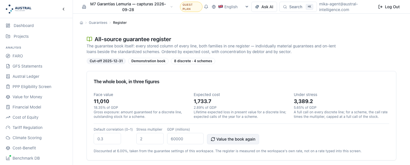
Figure 5.2 — The whole book, in three figures: face value 11,010 (18.35% of GDP), expected cost 1,733.7 (2.89%) and under stress 3,389.2 (5.65%) — §4.4's three figures, without typing a row. Above, the cut‑off date 2025‑12‑31, the demonstration‑book badge and the count 8 discrete · 4 schemes. Below, the three assumptions — correlation 0.30, stress ×2, GDP 60,000 — and the rate line with its provenance: "Discounted at 6.00%, taken from the guarantee settings of this workspace." (§5.1; Steps 1, 2, 3 and 6.) [note: GDP opens blank and is typed; the other two assumptions already open on §4's values.]
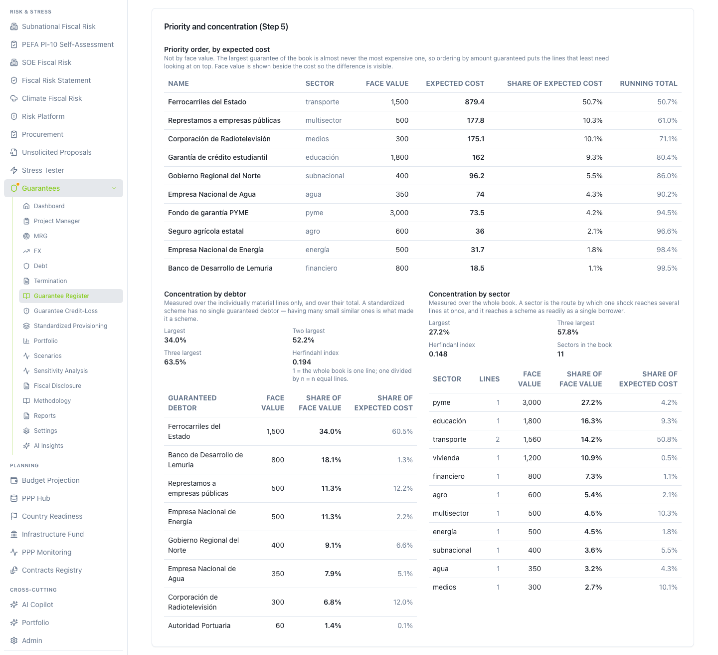
Figure 5.3 — Step 5, computed on the server and drawn on the screen. The order is by expected cost, not by face value, and the table puts the face value alongside so the difference shows: the SME guarantee fund is the book's largest row by face (3,000) and the seventh by cost (73.5), while Ferrocarriles del Estado is 1,500 of face and 879.4 of cost — 50.7% of the book. Below, the two concentrations: by debtor (largest 34.0%, three largest 63.5%, Herfindahl 0.194, measured only over the eight one‑off rows) and by sector (27.2%, 57.8%, Herfindahl 0.148 over eleven sectors, measured over the whole book). (§5.1; Step 5.) [note: the materiality table lists the ten largest of the twelve rows.]
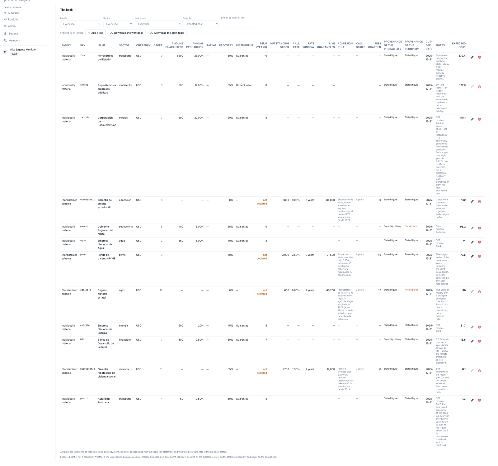
Figure 5.4 — The complete book. Filters by family, sector and instrument, search by name or key, five sort orders, and the twenty‑three columns the two calculation screens never showed: reporting order, instrument (Guarantee / On‑lending), rate window, live guarantees, admission rule, call series, provenance of the probability and of the recovery, cut‑off date and notes. The SME fund's row declares a nine‑year window and 21,500 live guarantees; the agricultural insurance one, two years and an admission rule widened in 2024 — in a rate cell the two looked identical. (§5.2; Steps 1 and 9.) [note: the table scrolls horizontally; the figure opens it whole. Two rows declare the probability taken from the sovereign library and one declares the recovery undeclared.]
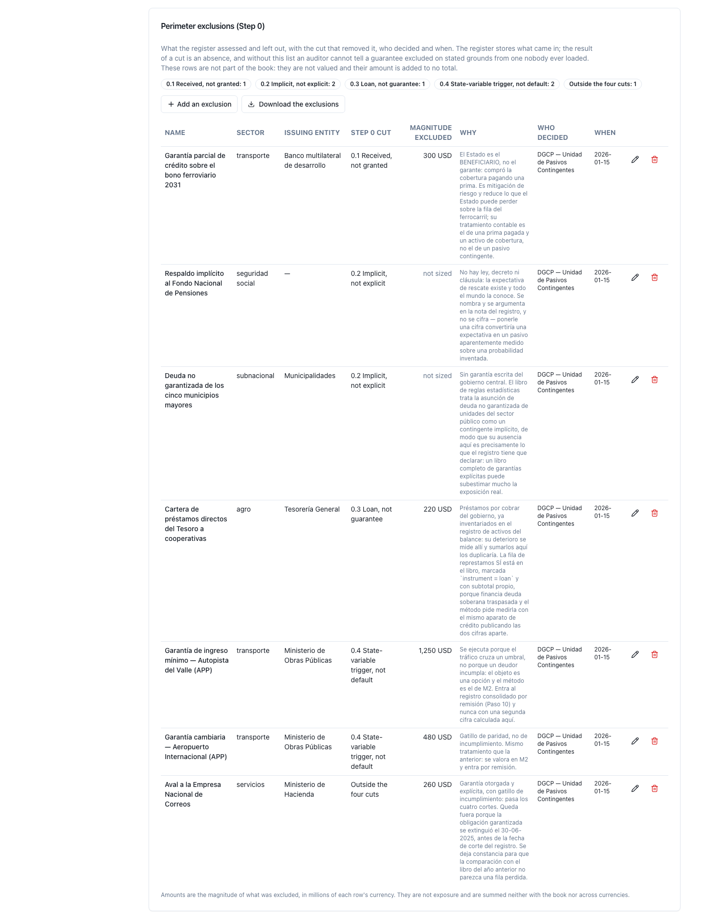
Figure 5.5 — The perimeter's record. Seven exclusions spread over the four Step 0 cuts — 1 received, 2 implicit, 1 loan, 2 state‑variable trigger — and one outside the four, each with its issuer, its magnitude — or "not sized", which is the right state for an implicit guarantee — the rationale for the cut in that particular case, who decided it and when. Step 0 cannot have a screen that reasons it; it can have, and now has, a screen that evidences it. (§5.1; Step 0.) [note: these rows are not part of the book: they are not valued and their amount is summed into no total.]
Route: …/guarantees/credit-loss. Product label: "Guarantee credit loss analyzer".
Input. A table of exposures with five editable columns — name, guaranteed amount, PD (0–1), term (years), recovery (0–1) — plus the default correlation, which opens at 0.20. The screen loads the workspace's saved register when it opens and says so: "Loaded from the workspace's guarantee register — cut‑off date …". If the workspace has no register yet, it opens with two starter rows and says, also, that they are not saved.
Output. Four headline figures — total exposure (EAD) and the three expected loss bases: annual, lifetime and lifetime in present value, the last with the discount rate printed alongside and the note "at X%, discounted from the base year" — a second row with VaR 95 / CVaR 95 and worst case / full call; the amber warning when some exposure did not declare a term, with how many out of how many; and the row‑by‑row detail with EAD, term, annual PD, lifetime PD, LGD and the three bases, ordered by lifetime expected loss in present value. At the foot, two notes: the formula with the conversion P = 1 − (1 − h)ⁿ and the correlation applied, and — literally — "Expected loss is not a provision… that is decided by the fiscal disclosure note, and on the LIFETIME probability."
Analyst's decision. The five columns of each row, the correlation and when to save. Three buttons: evaluate, save to the register and export the register.
It is worth pausing on what this screen runs, because it is the whole of Step 3 and was not always: there is a term column; the lifetime probability is computed and published row by row alongside the annual one; the three bases come out labelled; present value is discounted over the hazard path and from the base year; the rate comes from the workspace and is printed with its provenance; and the word "provision" appears in no output of the calculation. Step 3 of §3 is taught here with a screenshot and not with a warning.
Limits.
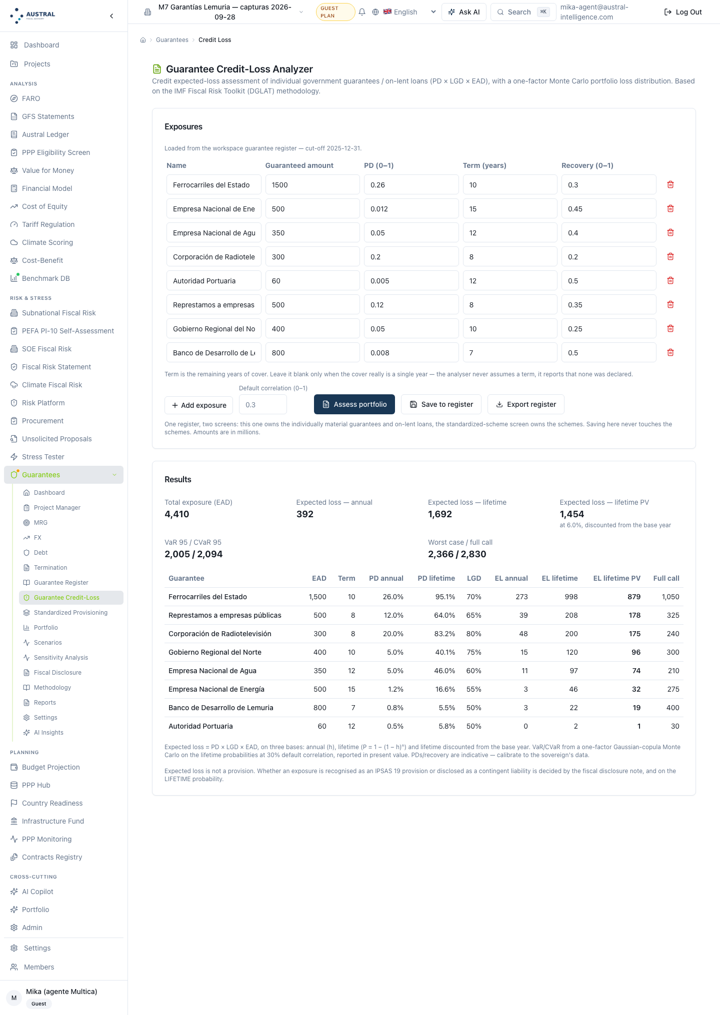
Figure 5.6 — Step 3 complete on one screen. Above, the eight exposures loaded from the register with their term and the notice "Loaded from the workspace's guarantee register — cut‑off date 2025‑12‑31". Below, total exposure 4,410 and the three labelled bases — annual 392, lifetime 1,692, lifetime PV 1,454, "at 6.0%, discounted from the base year" — the tail (VaR 95 / CVaR 95 = 2,005 / 2,094; worst case / full call 2,366 / 2,830) and the detail with annual PD and lifetime PD row by row. At the foot, the formula with the lifetime conversion and the note that expected loss is not a provision. (§5.1; Steps 1, 3 and 4.) [note: the figure's CVaR is 2,094 and §4's and the register's is 2,090.4: this screen runs 10,000 draws, not the workspace's 50,000 (limit 5). The amber undeclared‑term warning does not appear because all eight rows declare one.]
Route: …/guarantees/standardized-guarantee. Product label: "Standardized guarantee provision".
Input. A table of schemes with five columns — scheme, balance outstanding, call rate (0–1), recovery (0–1), fee income — the stress multiple (which opens at ×2) and GDP. Like the previous one, it loads the schemes saved in the register and declares it with their cut‑off date.
Output. Four headline figures — balance outstanding, expected calls with their percentage of GDP, net fiscal cost (less fees) and stressed calls with their multiplier — and the scheme‑by‑scheme detail with balance, expected calls, net cost and stressed cost. At the foot, the formula and the warning that recognition is decided by the disclosure note and not by this screen.
Analyst's decision. The five columns of each scheme, the stress multiple, the declared GDP and when to save.
Limits.
expected calls − fees, never stressed calls − fees, and the screen publishes no net under stress. It is rule (c) of Step 6 of §3, and it is exactly the finding a fund manager needs: fees do not rise with the calls. In the demonstration register, the social housing mortgage scheme has a net of 0.1 on average and 8.2 under ×2 stress, and the net for the whole set goes from 214.6 to 494.2 — all of which has to be computed outside the tool. [to be built]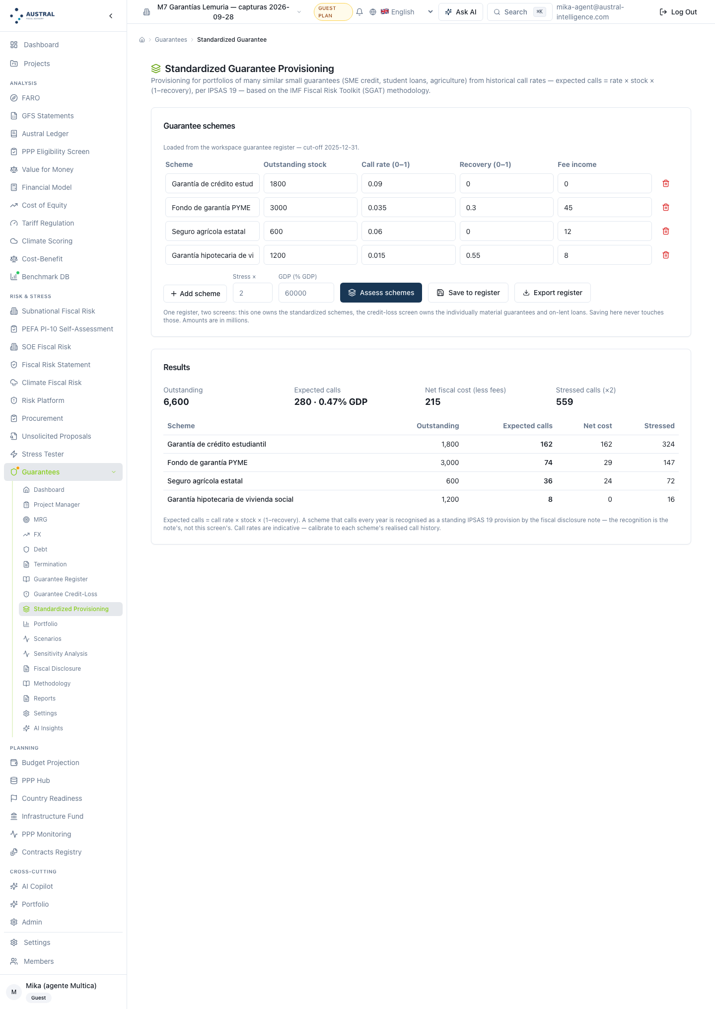
Figure 5.7 — The four schemes loaded from the register with their outstanding stock, their call rate, their recovery and their fee, and below outstanding 6,600, expected calls 280 · 0.47% of GDP, net fiscal cost 215 and stressed calls (×2) 559, with the scheme‑by‑scheme detail. The student credit guarantee, at 162 of 280, costs more than the other three schemes together and charges no fee. (§5.1; Steps 1, 3 and 6.) [note: the screen rounds to whole numbers — §4 publishes 279.6 · 214.6 · 559.2. The net is always the mean's: the social housing mortgage prints net 0 and stressed 16, and its net under stress — 8.2 — does not appear. Of the four percentages of GDP the calculation returns, the screen prints one.]
Route: …/guarantees/fiscal-disclosure. Product label: "Fiscal disclosure (IPSAS 19)".
It is the screen that has changed most, and the one that turns the register into a deliverable. Input: none on screen; the note is built over everything the workspace guarantees — the saved contract scenarios and the all‑sources register, each row in its own currency. Output: the headline ("n guarantees: p recognized as provisions, c disclosed as contingent liabilities"), the provenance line saying how many rows come from each source, the rate line with its provenance, four cards — recognized provisions in present value, contingencies: gross exposure, contingencies: estimated effect, and the count — the provisions table with present value and nominal sum, the contingencies table with gross exposure, estimated effect and the remote flag, the block of on‑lent loans and loans receivable under IPSAS 41 — outside the two IPSAS 19 tables and summed into neither — and the regulatory framework with the narrative the engine returns.
Four things this screen does today that are worth saying because they are recent:
Limits.
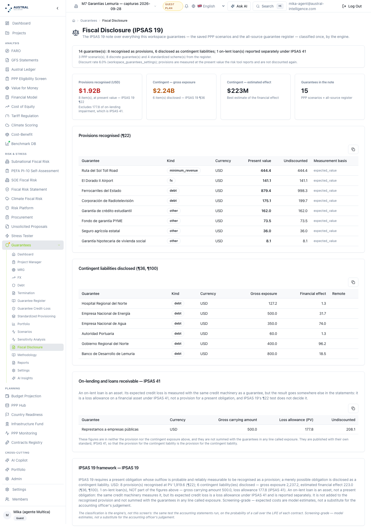
Figure 5.8 — The note over everything the workspace guarantees, with the provenance line that says so: 3 PPP scenarios, 8 discrete guarantees and 4 standardized schemes from the register. The eight recognized provisions of ¶22 and the six contingencies disclosed under ¶36 and ¶100 — and, below both blocks and summed into neither, "On‑lent loans and loans receivable — IPSAS 41": gross carrying amount 500.0 and loss allowance 177.8, with its reason written on the screen itself. The provisions card repeats it in its footnote: "Excludes 177.8 of on‑lending impairment, which is IPSAS 41." It is the closing rule of Step 7 executed by the product. (§5.1; Step 7.) [note: the screen does not publish the "remote" cut it applied, although the engine returns it and it is already unified at 5% across the product. And it does not let one choose which half comes in: the 1,334.1 provision of the all‑sources half — the method's figure (§4.7) — has to be taken from the exported workbook or subtracted by hand from the headline's 1,932.1.]
It is not a screen: it is the "Download the workbook" button on the register, which both calculation screens repeat as "Export the register". It produces a workbook with five sheets: the register as it is saved — with its cut‑off date, its rate and its provenance, the correlation, the stress multiplier and the number of runs with its seed in the header; credit loss with the three bases row by row, the total and the tail block; standardized schemes with balance, calls, fees, net and stressed; the IPSAS 19 note with its two tables, the on‑lending block under its own standard and its narrative; and the perimeter exclusions, which is what makes the book evidence of completeness and not only of what was valued. There is also an export in interchange format, with the twenty‑four columns of the Step 1 record, which goes back into the register after being edited in a spreadsheet.
Two points. The first, in its favour: the workbook's IPSAS 19 note sheet is the register's alone — 11 items, 6 provisions for 1,334.1 and the on‑lending apart — so the deliverable that is archived does publish the all‑sources note the screen does not let one isolate. The second, not: the workbook is labelled in English in any session language — the names of the five sheets and all their headers — and the download requires the workspace to be licensed: in a newly created workspace, which is born on the guest plan, the button returns a block. [to be fixed]
It is, today, the method's deliverable: what a ministry attaches to its fiscal risk statement and what an auditor opens.
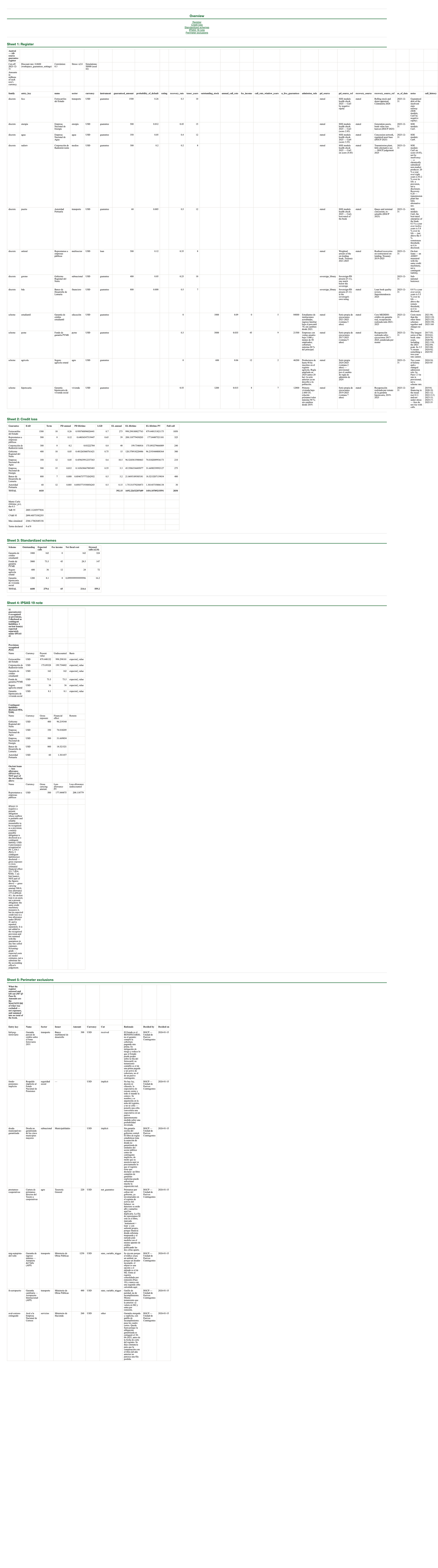
Figure 5.9 — The exported workbook, its five sheets and its assumptions header: cut‑off 2025‑12‑31, rate 0.0600 with its provenance, correlation 0.3, stress ×2, 50,000 runs with seed 42. Register with the twenty‑four columns of each row; Credit loss with the three bases row by row; Standardized schemes with balance, calls, fees, net and stressed; IPSAS 19 note over the register alone — 11 items, 6 provisions and the on‑lending apart under its own standard; and Perimeter exclusions, which is what makes the book evidence of completeness. (§5.1; Steps 1, 3, 4, 6 and 7.) [note: the workbook is labelled in English in any session language. The download requires a licensed workspace.]
Route: …/frs. The register enters the statement as two families — one‑off guarantees and standardized schemes — read directly from the workspace: nothing has to be pasted anywhere. It is shown once as a destination and referred out to M9, which is the manual for that screen.
Two points that belong to this manual and not to that one. The first: the collector values the register at zero correlation and without stress, deliberately — a portfolio's tail belongs to the assumptions of whoever declares it, and fixing a correlation on the statement's behalf would publish a CVaR nobody chose; whoever wants their own correlation in the statement sends the portfolio result explicitly, and that governs over the automatic reading. The second: the statement nets the explicit stock each state‑owned enterprise declares — guaranteed debt, on‑lendings and government loans — against the one‑off guarantee family, which is the no‑duplication rule of Step 10 executed by the product.
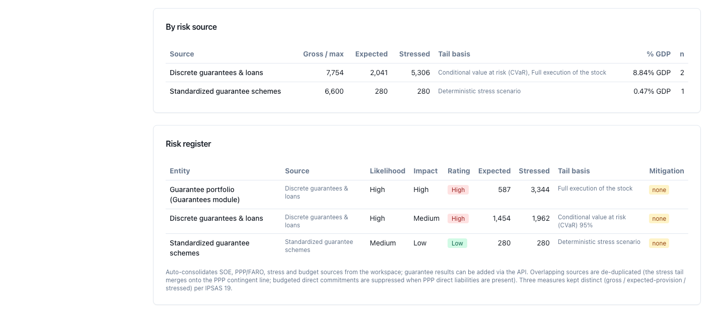
Figure 5.10 — The register enters the statement as two families — discrete guarantees & loans, standardized guarantee schemes — read from the workspace, each with its declared tail basis: conditional value at risk at 95% and full execution of the stock for the first, deterministic stress scenario for the second. The figures confirm what the text says: the collector values the register at zero correlation and without stress — expected 1,454 and stressed 1,962, which is the CVaR 95 of the one‑off portfolio at correlation 0 in §4.2; 280 and 280 for the schemes. The statement does not add tails measured on different laws without saying so: it labels them row by row. Referred out to M9 for this screen. (§5.1; Step 10.) [note: GDP is overridden to 60,000, as in §4.]
This is the question the manual has to answer precisely, because the answer has changed completely and because whether Step 9 is applicable depends on it.
Today there is a book, and there is a screen. The workspace stores an all‑sources guarantee register, one row per exposure, with two families in a single book — one‑off guarantees and schemes — and real columns, not a block of text: family, key, name, sector, currency, reporting order, guaranteed amount, annual probability, rating, recovery, instrument type, term, scheme balance, call rate, rate window, live guarantees, admission rule, call series, fees, provenance of the probability and of the recovery with their declared source, cut‑off date and notes. And a sister list: the perimeter exclusions, which are not rows of the book — they are not valued and sum into no total — but the record of Step 0.
There are three views of the same book, not two. The register screen (§5.1) shows it whole and edits any column. The two calculation screens are partial views: the credit loss one saves only the one‑off rows and the scheme one only the schemes, so that saving in one never overwrites what the other administers.
Nothing in the book is a result. Expected loss, the tail and the accounting classification are computed on read, with the same engines that run behind the screens. A saved row and a typed row cannot give different figures, and a change of engine does not leave the book with stale figures.
What the book makes possible, and the stateless calculation did not: a declared cut‑off date — and the warning that the book has two, that is, that it is half updated; the warning that the book carries more than one currency and the register stores no exchange rates; export to a workbook and to interchange format; a disclosure note over what is saved; automatic entry into the fiscal risk statement; Step 5 computed on the server — materiality and the two concentrations; the perimeter's record; and the cap of a thousand book rows and a thousand more exclusions, which is what makes the method applicable to a country register and not only to a workshop.
What there still is not.
The probability is typed in, and now where it comes from is declared. The register stores the provenance of the probability and of the recovery — stated, inherited from the form, sovereign library, other, or undeclared — and the source of each in free text, and both are edited in the row form. It is the half of Step 1.2 that used to live in a note: the screen also warns when a row has zero recovery without declaring where it comes from, because zero is not the neutral value but the severest possible assumption.
What is still missing is the shortcut. There is a sovereign rating to indicative annual probability library with eight countries, each with its rating, the table band, the probability and the declared source, and the calculation accepts a row coming in with a rating instead of a probability. The rating column is now editable in the register's row form, but it is a free‑text field: no screen offers the library — there is no country or rating selector — and nothing checks that what is typed is a rating the table knows. That is why the manual shows the programmatic query (§5.6) instead of inventing a screen. [to be built]
Both the rating‑to‑probability table and the sovereign library are declared indicative in the product itself, and this manual repeats the warning instead of softening it: they are corporate default studies, they are not calibrated for sovereigns or for state‑owned enterprises, and they have to be calibrated before being used with a client.
The scheme's call rate is typed in, and now the series it comes from is stored with it. The register has a call series column — one line per year, year:amount — a rate window in years, an admission rule and a live guarantees count. It is exactly what rule 1 of Step 3.2 asks for so that a rate is defensible: over Lemuria, the SME fund's declares nine years and the agricultural insurance's two, with the rule widened in 2024 — and in a cell the two looked identical. What the product does not do is compute the rate from the series or warn when the two do not agree: the rate is still a typed figure standing beside its evidence. [to be built]
Seven differences remain, and all of them are stated above under their screen. It is worth gathering them because together they draw the product's profile: the engine runs ahead of the interface, and the interface runs ahead of the navigation.
| What the method asks for | What the product does | Where |
|---|---|---|
| Guarantees and loans separated, with two subtotals | The book stores the instrument type and the register screen filters by it; the totals of all three screens still add them together | Step 0.3 · Step 2 |
| Structured correlation, or at least one declared by sector | A single scalar for the whole portfolio | Step 4 |
| A warning when the tail loses meaning for want of rows | Nothing | Step 4 |
| One tail per portfolio | Two: the register at 50,000 runs and the credit loss screen at 10,000, without saying so | Step 4 |
| Net of fees recomputed in the stress scenario | The net is always the mean one | Step 6 |
| Multi‑year projection of the scheme | One year | Step 3.2 · Step 6 |
| The contingent liability note on its own, without the contract scenarios | The exported workbook gives it; the screen does not let one choose | Step 7 |
And four the working index or the 25-09 drafting listed here and that are no longer differences: the annual probability with no term and no discounting; the "provision" label on expected loss; the contingent liability provision added together with the on‑lending impairment — the note now separates them, each under its own standard; and the absence of a register screen, which was the costliest of all. All four are corrected in the engine, on the screen and in the five language editions.
The vocabulary difference is corrected. In the Spanish interface the credit loss screen's subtitle said "préstamos on‑lending" while its footnote said "represtamos". Today the subtitle says "garantías gubernamentales individuales / represtamos", the scope note says "represtamos", the register screen labels the instrument "Represtamo" and the disclosure note titles its block "Represtamos y préstamos por cobrar". One word, M6's, on all four screens. This edition uses on‑lending, which is the term of the series in English and the one the Spanish edition renders with the house word.
What does remain of vocabulary [to be fixed]: several of the module's side‑menu entries stay in English even in a Spanish session — Guarantee Register, Fiscal Disclosure, Scenarios, Methodology, Project Manager — although the titles of those same screens are translated, and the values the engine computes for the accounting note print in English in a Spanish session (§5.0).
To the fiscal risk statement: automatic, reading the workspace's register, as described above. To accounting: the disclosure note uses the same classifier as the platform's accounting statements, so the note a ministry files and its balance sheet cannot disagree.
From the state‑owned enterprise module: [to be built]. That module publishes, enterprise by enterprise, the explicitly guaranteed stock, the on‑lendings and the government loans receivable — which are exactly the rows this register values. Today the continuity exists in the demonstration pack, where the register's first five rows are M6's five enterprises with their amounts, but there is no handover: in a real workspace those rows have to be typed in again, with the risk that the two readings drift apart. It is the handover that would add most value and the one that is missing.
From the contract register and to the budget: [to be built].
The no‑duplication rule is that of Step 10.2 and the product runs it at one point: the statement nets the explicit stock each state‑owned enterprise declares against the one‑off guarantee family, so that the same obligation does not come in twice. Today it also publishes it: the statement prints how much the register adds, how much was netted against the state‑owned enterprises and the net movement, and lists the seams between families with their verdict — including "not applicable (one of the two sides is missing)", which is the case of a workspace that has a register and no state‑enterprise portfolio. At the other points the rule is the analyst's, and the manual writes it down so that it is applied.
Everything the three screens do — and three things none of them does — is accessible with the account's session. In prose, without transcribing addresses:
The live list, as at 28-09-2026, ordered by what it costs:
Off the list — and it is worth saying, because an earlier manual's list is what the reader remembers — are the navigation to the two screens, the absence of a persistent register, the lack of an all‑sources demonstration pack, the disclosure note with no screen, the discrepancy of cuts between the engine and the browser, the register screen, the historical series of calls with its window and its admission rule, the declared provenance of the probability and of the recovery, the record of the Step 0 perimeter, the whole of Step 5 and — the most important for §7 — the contingent liability provision separated from the on‑lending impairment in the note. Five were open when this manual's working index was written; the last six were closed between 25 and 28 September, that is, after this section was called definitive. A manual of a living platform is written against a moving target, and the rule of the series is to say so with a date rather than to disguise it.
And a warning that is not the module's but that affects anyone following this manual: a newly created workspace is born on the guest plan, and the guest plan blocks downloads. One can seed Lemuria's register, value it, read the note and see all four screens; one cannot download the workbook. For the §5.1 deliverable one has to work in a licensed workspace.
| §3 step | Where it runs | Note |
|---|---|---|
| 0 Perimeter | Register (perimeter exclusions) | The argument is archive work; the record — what was assessed, which cut removed it, who decided it — does have a screen |
| 1 Inventory and partition | Register · Credit loss · Standardized schemes | Twenty‑three columns in the register's table; five on each calculation screen |
| 2 Face value | Register (the book's face value) · Credit loss · Schemes | No subtotal by instrument |
| 3 The three bases | Credit loss · Schemes · Register (expected cost) | Complete: term, lifetime probability, discounting from the base year |
| 4 The tail | Credit loss · Register | Scalar correlation; no degenerate‑tail warning; two different run counts |
| 5 Priority and concentration | Register | Complete: materiality by expected cost, concentration by debtor and by sector with Herfindahl |
| 6 Stress | Schemes (multiple) · Credit loss (full call) · Register (under stress) | No stressed net; no projection |
| 7 Treatment | Fiscal disclosure (IPSAS 19) | Liability provision and on‑lending impairment separated, each under its own standard; without being able to isolate the all‑sources half on screen |
| 8 Price and subsidy | — | It exists for the contract guarantees; not for these |
| 9 Ceiling and governance | Partial: Register (cut‑off date, provenance, export) | No version, no history, no ceiling |
| 10 Consolidation | Fiscal Risk Statement · programmatic valuation of the book | Netting with state‑owned enterprises executed and published by the product |
Everything described can be read and computed without registering: the guest workspace comes with Lemuria's complete register and the example's rate seeded, and it reproduces §4's figures with §4's assumptions printed on screen with their provenance. What the guest plan does not allow is saving, uploading or downloading — the §5.1 workbook requires a licensed workspace. The link is at the end of the manual.
And the handover note, which is the series': the client keeps the tool and the ability to operate it. §3's method is self‑contained and can be run without this platform; what the platform adds is that the register persists, that the figures are not computed twice in two ways, and that the note that is filed and the balance sheet that is published come out of the same classifier.
One has to begin with a concession, and it is not a courtesy. The two reference tools of this method are spreadsheets, and they are good ones: two spreadsheets of the International Monetary Fund's fiscal affairs department, published inside its fiscal risk toolkit, one for one‑off guarantees and loans and one for standardized guarantee schemes. §3's method can be run in them — in fact it came out of them. This manual is not written against those spreadsheets; it is written on the method those spreadsheets document.
This section's argument is a different and narrower one: what happens to a spreadsheet when it stops being a diagnostic instrument and becomes the annual register of a guarantee book. A diagnostic instrument is opened to answer a question about one guarantee, used for a day and filed. A register has a hundred one‑off guarantees arriving from the debt office, from three fund managers and from a budget annex; eight schemes whose call rates have to be reviewed every year; a cut‑off date; a reporting chain that ends in a signed financial statement and in a fiscal risk statement sent to Parliament; and an auditor who in three years' time will ask where a figure came from. None of those four things is a calculation problem; all of them are problems of base, provenance, invariants and versions, and none is solved with a better formula.
The ten failures that follow are not hypothetical. Each is presented the same way: where it occurs (which step of §3), what fails in the spreadsheet, what it costs measured over Lemuria's register from §4, and what the tool does instead. And several of them happened to the tool itself before being corrected; they are told that way, because the difference between a spreadsheet and a program is not that the program does not get it wrong, but that when it does it leaves a trace, it is corrected once for all hundred guarantees, and a test remains that stops it coming back.
Where it occurs. Step 2, and it is the failure that orders all the others.
What fails in the spreadsheet. The spreadsheet adds up the column of guaranteed amounts, calls it "the State's exposure" and publishes it. It is the most natural operation in the world: the amount is written down, the guarantee was signed by the Treasury, the sum is correct. Everything else — the probability that it is called, the term over which it can be called, what would be recovered if it is — is in other columns that do not make the headline, if they are there at all.
What it costs in Lemuria. The same register admits four figures, all of them true:
| Reading | Amount | % of GDP |
|---|---|---|
| Face value of the book (the spreadsheet's) | 11,010 | 18.35% |
| Maximum exposure on a full call, net of the declared recovery | 3,389.2 | 5.65% |
| Lifetime expected cost, in present value | 1,733.7 | 2.89% |
| Expected cost for the year | 671.8 | 1.12% |
The first is 6.35 times the third and more than sixteen times the fourth. None is false and each answers a different question: the first is a permission, the second a scenario, the third a liability and the fourth a budget line. The damage of publishing only the first is not that it exaggerates the risk — although it does, and GFSM 2014 says so in the footnote to its ¶7.255: the nominal value approach "offers no information on the likelihood of the contingency occurring and it may overstate the possible risk". The damage is that it answers none of the questions a ministry has to answer: one cannot budget on 11,010, one cannot provision on 11,010 and one cannot size a fund on 11,010.
And there is a finer confusion inside the same failure, which is the one that distinguishes a good register from a correct one: the maximum exposure is not the face value. It is 3,389.2 and not 11,010, because the maximum exposure assumes the declared recovery. A spreadsheet that publishes face value as "maximum possible loss" is exaggerating by a factor of 3.25, and doing it with a prudent face on.
What the tool does. It publishes the three bases together and labelled in the same output, with the discount rate and its provenance alongside, and it offers no operation that adds them. The label is not cosmetic: it is what obliges whoever copies the figure into a report to say which one they copied.
Where it occurs. Steps 3 and 7. It is the most expensive error in the book and the hardest to see.
What fails in the spreadsheet. A cell with a probability, and a comparison. The probability comes from a rating table — every rating table publishes annual probabilities, because they come from one‑year default studies — and the comparison is with the IPSAS 19 threshold, the 0.5 of its ¶31. The formula is correct, the table is real, the threshold is the standard's. What is missing is a conversion none of the three pieces asks for: the obligation does not last a year, it lasts the term of the guarantee, and the probability the recognition test needs is that of there being some call over that term.
What it costs in Lemuria. It is the largest measurement in this section.
| Test on the annual probability | Test on the lifetime probability | |
|---|---|---|
| Rows recognized as a liability provision | 4 | 6 |
| Contingent liability provision | 279.6 | 1,334.1 |
| Does the 1,500 guarantee to the insolvent railway come in? | no (26.0% < 50%) | yes, 879.4 |
| Does the mortgage guarantee of 8.1 come in? | yes | yes |
| The two line items added together, with the on‑lendings inside | 279.6 | 1,512.0 |
×4.77 on the liability provision, which is the comparable comparison — whoever adds the provision to the on‑lending's loss allowance gets 279.6 against 1,512.0, ×5.41, but that addition puts 177.8 of impairment of an asset at only one of the two ends (§4.7). And the detail that turns the figure into an argument: with the test on the annual probability, the guarantee with the highest expected cost in the whole register stays off the balance sheet while one of 8.1 comes in. Not because anyone miscalculated: the railway's 273.0 of annual cost is correctly multiplied, and the 26% is the right number from the right table. Because a twelve‑month probability was compared with the threshold of a ten‑year obligation, and the same standard that sets the threshold (¶22 with ¶31) measures the provision at the expected value of the obligation (¶44 with ¶47 and ¶53), not of one year of it. If the measurement is lifetime, the test has to be on the same base.
The conversion that separates the two readings fits on one line: P = 1 − (1 − h)^n, and on the railway it gives 1 − (1 − 0.26)^10 = 0.951. A spreadsheet can have it. What a spreadsheet does not have is the guarantee that it is in all hundred rows, in the right column, and that nobody dragged it wrongly in row 74.
What the tool does. The conversion is not an optional column: it is part of the calculation, it is published alongside the annual probability in every row, and the accounting classifier runs on the lifetime one and not on the annual one because it has no access to the other. The tool made this error until recently — it published and classified on the annual probability — and correcting it moved §4's example from 279.6 to 1,334.1 of liability provision in one go, in the engine, on both screens and in the five translations. It is exactly this section's argument: an error of base in a spreadsheet is corrected spreadsheet by spreadsheet, and nobody knows how many were left uncorrected.
Where it occurs. Step 3, in the result column.
What fails in the spreadsheet. Two omissions that travel together. The first: there is no term column, because the expected loss formula does not ask for one — PD × severity × exposure is computed without knowing how long the cover lasts. The second: there is no discounting, because a column that multiplies three cells has nowhere to put it. The result is a column of expected cost that is not comparable across rows — a guarantee at seven years and one at fifteen appear in the same unit and are not in one — and is not summable across the register, because adding fifteen years of one and seven of another without declaring the horizon produces no known magnitude.
What it costs in Lemuria.
| Base | One‑off block | % of GDP | Multiple over the annual |
|---|---|---|---|
| Annual, with no term and no discounting (the spreadsheet's) | 392.2 | 0.65% | — |
| Lifetime, undiscounted | 1,692.2 | 2.82% | ×4.32 |
| Lifetime, in present value at 6% | 1,454.1 | 2.42% | ×3.71 |
From 392.2 to 1,454.1, and the distance is not spread evenly: it is contributed almost entirely by the handful of rows with a long term or a high probability. The railway goes from 273.0 to 879.4; the broadcaster from 48.0 to 175.1; the on‑lending from 39.0 to 177.8. All three are the three most expensive in the book and all three are the ones the annual reading understates most, which is no coincidence: the annual base compresses precisely the rows the register exists to find.
And there is a third figure worth looking at because it is the one a reviewer asks for: the difference between 1,692.2 and 1,454.1 is the discounting, 14.1%, and it is smaller than the error of base by an order of magnitude. It is the hierarchy of Step 3's three levers, measured:
| Lever | Effect on the lifetime expected cost in PV |
|---|---|
| The base of the probability (annual → lifetime) | +270.8% |
| The recovery, ten percentage points | −14.4% |
| The discount rate, from 6% to 8% | −4.3% |
A reviewer arguing about the rate and not about the base is arguing about the lever that moves 63 times less.
What the tool does. The term is a field of the row; discounting is applied over the hazard path year by year — (1−h)^{t−1}·h, surviving each earlier year — and from the base year, which is not discounted, so that a present value from this register can be added to one from another manual in the series without asking from which year each clock runs. And what it does not do, which is just as important: it does not assume a term when one is missing. With no term declared the two lifetime bases collapse onto the annual one and the result says that the term was not declared. A term assumed by default is an invented figure with the appearance of a calculation, and a spreadsheet that puts 1 in the empty cell produces exactly the annual column above without anyone noticing that it did.
Where it occurs. Step 3, at data entry.
What fails in the spreadsheet. An empty cell the formula reads as zero. Severity is 1 − recovery, so a blank recovery gives severity 1: the harshest hypothesis there is. Everything guaranteed is lost, neither collateral nor a claim against the debtor is recovered. And it produces no signal: the result is higher, and a higher result in a risk register looks like prudence. Nobody audits a figure for being conservative.
What it costs in Lemuria.
| Recovery assumption | Annual expected cost | Lifetime cost in PV | Maximum exposure |
|---|---|---|---|
| Declared, row by row (the register) | 392.2 | 1,454.1 | 2,830.0 |
| Zero on every row (the empty cell) | 560.2 | 2,097.7 | 4,410.0 |
+44.3% in the lifetime expected cost, without a single cell being wrongly computed. And on the maximum exposure the effect is exact and revealing: with zero recovery the maximum exposure coincides with face value (4,410), so the two figures §6.1 insists on not confusing become the same one, and the spreadsheet that was confusing them stops being wrong — by the wrong route.
On the schemes the same defect weighs less and in the same direction: 279.6 → 321.0 (+14.8%), and the net 214.6 → 256.0. It weighs less because two of the four schemes declare zero recovery, and declare it rightly: there is no collateral to enforce over a professional qualification or over a lost harvest. Which shows the other half of the argument, the important one: a declared zero recovery and a default zero recovery are the same figure and are not the same data. One is a judgement with its basis; the other is a cell nobody filled in. A register has to be able to tell them apart and a spreadsheet cannot, because in a spreadsheet the two look identical.
What the tool does. Recovery is a field with an explicit value on every row of the register, and the file the register exports brings the column and brings the notes field where its provenance goes. It is a partial correction and the manual says so: the tool does not oblige anyone to declare the provenance and does not distinguish a written zero from an inherited one, so the discipline is still the analyst's. What it does prevent is the zero propagating without being written down.
Where it occurs. Step 0, the perimeter's fourth cut; the damage appears in Step 2 and in Step 7.
What fails in the spreadsheet. A single table and a single total. The two reference tools handle government guarantees and loans on the same board — it makes sense: the credit arithmetic is the same — and the spreadsheet that copies them inherits the shared table without inheriting the distinction. The result is an "exposure" total that adds a conditional liability to an impaired asset.
What it costs in Lemuria.
| Face value | Annual expected cost | Lifetime cost in PV | Full call | |
|---|---|---|---|---|
| Guarantees (7 rows) | 3,910 | 353.2 | 1,276.3 | 2,505 |
| On‑lendings (1 row) | 500 | 39.0 | 177.8 | 325 |
| Total the spreadsheet publishes | 4,410 | 392.2 | 1,454.1 | 2,830 |
The loan is 11.3% of face value and 12.2% of the lifetime expected cost in present value. It is not a decimal error: it is an eighth of the figure published as contingent exposure that is not a contingent exposure. And the damage does not stop at the total. It has three branches.
It double counts with the asset register. The 500 of on‑lendings is, or should be, on the State's balance sheet as a receivable. Adding it to the contingent exposure counts it twice in the same financial statement, once as an asset and once as a liability risk.
It enters the portfolio tail. In §4.5's loss distribution, the on‑lending row contributes 277.7 of booked loss and is inside the atom that forms the VaR 95. A fund sized on that CVaR is reserving against the impairment of an asset as though it were a guarantee payout.
And it ends up in the wrong accounting line item. The IPSAS 19 test, applied to the on‑lending row, leaves it on the recognized side — its lifetime probability is 64% — and a spreadsheet totals it with the provisions. The figure is correct; the line item is not: the impairment of a receivable is a loss allowance on an asset, not a provision. Lemuria's contingent liability provision is 1,334.1, not the 1,512.0 that adding the two gives, and the difference is exactly that 177.8. The tool publishes them separately today, each under its own standard; it added them into a single total until 25 September 2026 (§4.7).
What the tool does. The register stores the instrument type on every row, the screen preserves it on editing — so that changing a probability does not silently turn an on‑lending into a guarantee — and the valuation receives it. But it is a half correction and that has to be said: the output adds the two into a single total of exposure and into a single portfolio tail, without publishing the two subtotals of the table above. Until it publishes them, that table is made alongside.
Where it occurs. Step 4.
What fails in the spreadsheet. A column of expected losses, a sum cell, and the conviction that this is the portfolio. It is, for one thing: the sum of the expected losses is the mean of the portfolio's loss, exactly, and no correlation changes it. The problem is that the mean is not the question. The question is how much has to be kept aside for the year in which several are called at once, and that depends on a parameter that appears in no mean.
What it costs in Lemuria.
| Correlation | Mean | VaR 95 | CVaR 95 | Simulated maximum |
|---|---|---|---|---|
| ρ = 0 (the sum's) | 1,454.6 | 1,844.1 | 1,961.8 | 2,366.2 |
| ρ = 0.30 | 1,454.1 | 2,005.1 | 2,090.4 | 2,366.2 |
The mean is the same — 1,454 in both cases — and the CVaR 95 rises by 6.6%. Said as whoever sizes the fund needs it: the excess of the CVaR over the mean is 636.3 at ρ = 0.30 and 507.7 at ρ = 0, so assuming independence cuts the fund by 20.2% — 128.6 of the 636.3 is put there by the correlation assumption, and that assumption is visible in none of the figures the spreadsheet publishes.
The simulated maximum, by contrast, is identical in both cases: 2,366.2, the full call in present value. With eight exposures of high lifetime probability, the scenario in which everything is called is reached even without any correlation at all. What the correlation changes is not where the tail ends, it is how frequent and how fat it is. It is a distinction worth making slowly, because intuition says the opposite: correlating does not make the worst case worse, it makes the bad cases worse.
What the tool does. It simulates the joint distribution with a one‑factor model over the lifetime probabilities, reported in present value on the same base as the analytical total, and publishes mean, VaR, CVaR and maximum. A spreadsheet does not simulate 50,000 runs of eight correlated variables and remain a spreadsheet — and the two reference tools, honestly, do not try: the portfolio distribution is a house addition and not an output of the source.
With two declared limits. The correlation is a single scalar — no pairwise matrix and no macro factor, which the same module does offer for the contract portfolio, so the assumption is worse here than there — and it is a house convention and not an estimate, because an all‑sources guarantee book does not have the series of joint calls that estimating it would require. And with few exposures the distribution has few steps: with Lemuria's eight rows the VaR at ρ = 0.20 and at ρ = 0.30 is the same number, because the 95th percentile falls in the same atom — the "six of the eight are called" scenario — and the screen does not warn. The manual recommends reading the CVaR and explains why; a spreadsheet has neither the problem nor the warning.
Where it occurs. Step 1, before any formula.
What fails in the spreadsheet. A single sheet with a single formula. If the sheet is the one‑off guarantee one, the scheme comes in as a large exposure with a probability from a rating table. If the sheet is the scheme one, the one‑off guarantee comes in as a balance with a call rate. In both directions the arithmetic runs without protest, because both formulas accept the same data types.
What it costs in Lemuria, in both directions. The comparison is made over five years, which is the horizon to which the register projects its schemes.
(a) The scheme valued as a large guarantee — its annual call rate is taken for a probability of default and converted to a lifetime probability:
| Scheme | Correct (5-year flow) | Valued as one‑off | Error |
|---|---|---|---|
| Student credit guarantee | 810.0 | 676.7 | −16.5% |
| SME guarantee fund | 367.5 | 342.7 | −6.8% |
| State agricultural insurance | 180.0 | 159.7 | −11.3% |
| Social housing mortgage guarantee | 40.5 | 39.3 | −3.0% |
| Total | 1,398.0 | 1,218.4 | −12.8% |
It understates, and the reason is exactly the opposite of §6.2's: the conversion to lifetime probability caps at 1, because it describes an event that can occur only once. A pool of twenty‑six thousand mortgages that calls 1.5% every year is not an event that occurs once: it occurs every year and the probability of its occurring does not accumulate, it repeats. And the error is larger where the rate is higher — student credit, −16.5% — that is, in the most expensive scheme in the book.
(b) The one‑off guarantee valued with a historical call rate — its annual probability is applied to the balance every year, with no survival:
| Guarantee | Correct (lifetime) | Valued as a scheme | Error |
|---|---|---|---|
| State Railways | 998.3 | 2,730.0 | +173.5% |
| Public Broadcasting Corporation | 199.7 | 384.0 | +92.3% |
| Northern Regional Government | 120.4 | 150.0 | +24.6% |
| Total of the seven guarantees | 1,484.1 | 3,463.7 | +133.4% |
It overstates, and here the reason is that the scheme formula has no survival: it charges 26% of 1,500 ten years running, as if the railway could default ten times. A debtor can only default once, and after the first there is nothing left to call.
The two measurements together are the step's argument: there is no conservative formula and aggressive formula. There are two formulas describing two different objects, and using the wrong one goes wrong in whichever direction falls to it — 13% below or 133% above — depending on which of the two objects is in front of you. The partition in Step 1 is not a presentational preference: it is what decides which arithmetic applies.
What the tool does. Two families in a single register, with two engines and two screens, and the family is a field of the row. A scheme row cannot reach the credit engine or the other way round, and the valuation of the complete book calls both and presents the two results separately before aggregating them with their label. What the tool does not do is the partition test: the four questions of Step 1 are answered by the analyst, and in particular the fourth — is there an own history of calls? — has neither a field nor a validation, because the register stores the rate and not the series it came from.
Where it occurs. Step 6.
What fails in the spreadsheet. A subtraction in the stress scenario row. The calls are multiplied by the stress factor — the spreadsheet does that right — and then the fee column is subtracted from them, and it is the same column as the base scenario's. Fees do not rise with the calls: a fee is charged on the guaranteed balance, not on what is paid out. The subtraction is arithmetically impeccable and describes a world that does not exist.
What it costs in Lemuria.
| Base scenario | ×2 stress | |
|---|---|---|
| Expected calls of the four schemes | 279.6 | 559.2 |
| Fees | 65.0 | 65.0 |
| Net fiscal cost | 214.6 | 494.2 |
The net goes from 214.6 to 494.2, and a spreadsheet subtracting 130 of stressed fees would publish 429.2. But the damage is not in the aggregate: it is in the individual row, because that is where the conclusion is inverted.
The social housing mortgage guarantee is the best scheme in the book: 1,200 of balance, a call rate of 1.5%, a recovery of 55% because there is a house behind it, expected calls of 8.1 and fees of 8. Its net fiscal cost is 0.1 — self‑financing to the last cent, exactly the scheme a manager presents as proof that the programme is well designed. With the ×2 multiplier the calls go to 16.2 and the fees are still 8: the net goes from 0.1 to 8.2, eighty‑two times. A scheme that on average costs the Treasury nothing costs it, in the stress scenario, its entire provision. It is the figure a guarantee fund manager needs and it is the one the badly made subtraction erases.
What the tool does. It stresses the calls. And it does not recompute the net — the net fiscal cost it publishes is always the mean one, and there is no stressed net in the output. So this failure, in the concrete version this section measures, is committed today by the tool as well, and the two figures of the table above are computed alongside. It is told that way, with the finding open and named in §5, because this section's argument was never that the program does not get it wrong: it is that when it does there is a single formula to correct and a test that stops it coming back, and not eight spreadsheets in four directions of which nobody has the inventory.
And a second half of the same failure, smaller and easier: the engine computes four figures as a percentage of GDP — expected calls, stressed, balance and net cost — and the screen prints one. A register wanting to compare its scheme book against a fiscal ceiling needs all four, and today three of them exist and are not shown.
Where it occurs. Step 2 for the thresholds, Step 1 for the rates, Step 9 for the file.
What fails in the spreadsheet. Three things that are the same thing. The probabilities of a hundred guarantees come from a rating table pasted into a helper sheet, with no source, no year and no warning that corporate default tables are not calibrated for sovereigns or for state‑owned enterprises. The call rates of eight schemes are numbers somebody typed in, without the series they came from or the window over which they were computed. And the file has no version: it is called guarantee_register_v3_final_REV2.xlsx, it has the modification date of whoever opened it last and no cut‑off date at all for the data it contains.
What it costs in Lemuria. What it costs is not an error: it is the impossibility of defending a figure. And it is measured by moving a single step of the rating table on the largest guarantee in the book. The indicative table the method publishes runs from 0.01% for the best grade to 26% for the worst before default, and the railway is scored at that last one:
| The railway's step | Annual PD | Lifetime PD | Lifetime cost in PV | Treatment |
|---|---|---|---|---|
| The register's (the worst grade) | 26.0% | 95.1% | 879.4 | recognized provision |
| One better | 5.0% | 40.1% | 336.8 | disclosure in the note |
| Two better | 1.2% | 11.4% | 93.7 | disclosure in the note |
One step changes the expected cost by 61.7% and takes the largest provision in the book off the balance sheet: the register's contingent liability provision would fall from 1,334.1 to 454.7. Nobody has to make a mistake for that to happen: it is enough that the table comes from a corporate default study of another economy, or that whoever scored the enterprise read the previous year's record. And the question the auditor will ask in three years' time — "where did the 26% come from?" — has no answer in a helper sheet with no source.
The same arithmetic holds for the schemes' call rates, and there the effect is linear and direct: the student credit rate is 9.0% and produces 162.0 of the block's 279.6 expected calls. One percentage point of that rate is 18 a year. Over what window that 9.0% was computed is written nowhere in the register, and the difference between a rate computed over nine years and one computed over the two years of the pandemic is not visible in the cell.
What the tool does. Less than it should and more than it seems. Every row of the register has a cut‑off date, currency, sector, instrument and a notes field, and the file it exports brings them all, so that the published figure travels with the state of the book that produced it. The rating table comes declared as indicative and to be calibrated in the product itself, and the manual repeats that warning instead of softening it. And the discount rate is published alongside its provenance in every result.
What is missing, and is declared: there is no historical series for the scheme, so the window of its rate has no field; there is no compulsory provenance for the probability or for the recovery; and there is no version of the register with the difference against the previous year explained by cause, which is what Step 9 asks for and what turns a register into an auditable document. A register that cannot say why its figure changed from last year is no better than the spreadsheet: it is a spreadsheet with a database.
Where it occurs. Step 10.
What fails in the spreadsheet. Nothing, inside the spreadsheet. The failure is that the spreadsheet is the end of the road. §4's figures have eleven different destinations — the balance sheet, the note to the financial statements, the statistical memorandum item 6M61, the statistical balance sheet, the year's budget, the fiscal risk statement, the sizing of the fund, the subsidy report, the concentration limit — and each one needs a different view of the same book, squared with the others. A spreadsheet produces them by copying and pasting, and every copy is an opportunity for one of the three readings of §4.7 to stop reconciling with the other two.
What it costs in Lemuria. The reconciliation in §4.7 has three columns that do not coincide and should not: the accounting one recognizes 1,334.1 of liability, the statistical one measures 1,248.4 of scheme liability plus 3,910 of memorandum, and the budgetary one 632.8 for the year. A reader who sees those three figures in three different documents, without the table that relates them, is going to conclude that two of the three are wrong. The no‑duplication rule has the same problem and is more dangerous: the 2,710 of guaranteed debt of the five state‑owned enterprises appears inventoried in one manual and valued in another, and adding them — which is what any consolidation by copying does — duplicates half the book.
What the tool does. It stores the register with its cut‑off date, values it from the inputs in a single call — so that a saved book cannot disagree with the engine that values it, because no column of the register is a result — assembles the disclosure note over the same book, exports the set in a five‑sheet file and delivers the two families to the fiscal risk statement. And what is missing, declared: there is no automatic handover from the state‑owned enterprise module — which publishes the stock this manual values — nor to the budget, so the two borders where duplication can occur are still manual.
| # | Failure | Step | What it costs, measured |
|---|---|---|---|
| 6.1 | Face value called exposure | 2 | 11,010 against 1,733.7 of lifetime expected cost in PV: ×6.35. The maximum exposure is 3,389.2 and not 11,010 |
| 6.2 | The annual probability against a lifetime threshold | 3, 7 | Liability provision 279.6 against 1,334.1: ×4.77. The 1,500 guarantee to the railway, off the balance sheet |
| 6.3 | The expected cost with no term and no discounting | 3 | 392.2 against 1,454.1: ×3.71. The base moves 63 times more than the rate |
| 6.4 | Recovery at zero by default | 3 | 1,454.1 → 2,097.7: +44.3%. And the maximum exposure becomes the face value |
| 6.5 | Guarantees added to loans | 0, 2, 7 | 500 of asset inside 4,410 of contingent exposure: 12.2% of the expected cost, and the liability provision is 1,334.1 and not the 1,512.0 of adding the two line items |
| 6.6 | The portfolio as a sum of independents | 4 | CVaR 1,961.8 → 2,090.4. The fund, 507.7 → 636.3: independence cuts it by 20.2% |
| 6.7 | The scheme treated as a guarantee and the guarantee as a scheme | 1 | −12.8% one way, +133.4% the other. On the railway, 2,730.0 against 998.3 |
| 6.8 | The net of fees that is not stressed | 6 | Net 214.6 → 494.2. A self‑financing scheme (0.1) comes to cost 8.2: ×82 |
| 6.9 | Thresholds and rates with no provenance, file with no version | 1, 2, 9 | One rating step: −61.7% on the largest row, and the register's liability provision from 1,334.1 to 454.7 |
| 6.10 | The register that has nowhere to go | 10 | Eleven destinations, three readings that do not coincide and should not, and 2,710 that are duplicated if someone adds them |
Three of the ten — 6.2, 6.3 and half of 6.4 — were committed by the tool itself and are corrected. One — 6.8 — is committed today and is named in §5 with the finding open. Two — 6.5 and 6.7 — are half corrected: the data is in the register and the subtotal is not in the output. All ten are told by the same yardstick, because a manual that listed only other people's failures would be a brochure.
Four things, and they are not rhetorical concessions.
Understanding one guarantee. To see how the expected loss of one guarantee moves when the recovery is changed, there is nothing better than a cell and a key. Table 4.8 of §4 — the sensitivity to recovery — is easier to understand in a spreadsheet than on a screen, and whoever has not done it by hand once does not understand what the screen is showing them.
Exploring a method before programming it. The two reference tools are spreadsheets for a good reason: a spreadsheet is a method one can read. The reader can open the formula, follow it, argue with it and correct it, and that is exactly what a ministry needs in order to adopt a method it will later have to defend. A program hides the formula; a spreadsheet publishes it.
Teaching. A two‑day workshop on guarantee valuation is done in a spreadsheet, and this manual recommends doing it.
Diagnosing a new guarantee before a register exists. A ministry asked for a guarantee on Thursday does not need a database: it needs PD × severity × exposure, the term conversion and the break‑even premium, and all three fit on one sheet.
What is not done in a spreadsheet is the register: a hundred rows arriving from four places, with a cut‑off date, a probability base that has to be the same in all hundred, three bases published together, a simulated tail, a disclosure note an auditor is going to sign, eleven destinations that have to reconcile and a version explaining why this year's figure is not last year's. The border between the two is sharp and worth stating in one line: the spreadsheet is better for understanding one guarantee; the register, for governing a guarantee book and defending its number before an auditor.
No figure in this chapter is new: all of them come from §4's example, and all from the same run of the engine on Lemuria's register. The correspondence, so that a reviewer can go and find them:
| § | Figures | They come from |
|---|---|---|
| 6.1 | 11,010 · 3,389.2 · 1,733.7 · 671.8 | §4.3, table 4.3 |
| 6.2 | 279.6 · 1,334.1 · ×4.77 · 1,512.0 (the two line items added together) · ×5.41 · 879.4 · 273.0 · 95.1% | §4.7, table 4.15 and box 4.4.1 |
| 6.3 | 392.2 · 1,692.2 · 1,454.1 · the three levers | §4.4, table 4.6 and the two sensitivities |
| 6.4 | 560.2 · 2,097.7 · 4,410 · 321.0 · 256.0 | §4.4, table 4.8 |
| 6.5 | 3,910 / 500 · 353.2 / 39.0 · 1,276.3 / 177.8 · 277.7 · 1,334.1 | §4.1, §4.4 table 4.6, §4.5 table 4.10, §4.7 |
| 6.6 | 1,961.8 · 2,090.4 · 636.3 · 507.7 · 2,366.2 · 2,005.1 | §4.5, tables 4.9 and 4.11 |
| 6.7 | 1,398.0 / 1,218.4 · 1,484.1 / 3,463.7 · 2,730.0 | measured over the same register at five years |
| 6.8 | 214.6 · 494.2 · 0.1 → 8.2 | §4.6, box 4.6.1 |
| 6.9 | 336.8 · 93.7 · 454.7 · 162.0 of 279.6 | measured by moving the railway's rating |
| 6.10 | 1,334.1 · 1,248.4 · 3,910 · 632.8 · 2,710 | §4.7 table 4.17 and §4.9 |
The two rows that do not refer to a §4 table — 6.7 and 6.9 — are measurements made for this section over the same register and with the same engines: the miscategorization of the two families and the step of the rating table. They are computed in the same run as everything else, and are recomputed with it.
Every reference was consulted on 24 September 2026, except reference 24, downloaded again and extended on 25-09-2026 for the definitive box 4.8, and 24b, opened that same day. Unless otherwise indicated, each document was read in its official version — a PDF downloaded from the publisher's site. ✔ = verified by direct reading for this manual · ✔M2 / ✔M6 = verified for that manual of this series and not re‑read · ✔p = verified in the publisher's own presentation material, without reading the user guide of the product cited — which in the case of references 1 and 2 is not published, it is not pending opening · PV = to be verified (existence confirmed; the datum indicated is checked against the document before being cited in the body). Where a document was read through another reference, it is said. For this English edition the three accounting standards and the legal instrument of reference 19 were opened again and read directly in their official English text; the notes on those entries record what that check settled and what it did not.
EL = PD × LGD × EAD and of the asset correlation treatment. PV edition and paragraphs. It is cited as the provenance of the identity, not as a standard applicable to the public sector — the distinction is written into §2.4 and is not a formality: no bank capital requirement binds a ministry of finance.24b. Chile — Decree Law No. 1,263 of 1975, on the Financial Administration of the State, art. 2 (the definition of "public sector" on which reference 24's perimeter rule depends) and art. 40 (the mandate for the annual report). [to be verified] — the text of the law on the National Congress Library site (https://www.bcn.cl/leychile/navegar?idNorma=6536) returns HTTP 401 and could not be read directly. What §4.8 asserts about art. 40 and about the scope of the "public sector" is taken from the literal quotation and the summarized enumeration made by the Dipres report itself (reference 24, Presentation and ch. II.1), and is declared as such. What remains unresolved, and is flagged in §4.8: whether a regional government falls inside that "public sector". The report's enumeration — Central Government, National Congress, Judiciary, Comptroller, "among others" — neither names them nor excludes them.
25. Colombia — Law 448 of 1998, "adopting measures in relation to the management of the contingent obligations of State entities". Art. 1 (entities must include in their debt service budgets the appropriations to cover the possible losses of the contingent obligations they carry; paragraph: a contingent obligation is a pecuniary obligation subject to a condition); art. 2 (creation of the Contingency Fund of State Entities); art. 3 (purpose); art. 4 (the contributions are deemed executed on being transferred and are refunded only "when it is definitively established that the anticipated risks have not materialized"); art. 5 (resources); art. 6 (the Directorate General of Public Credit approves the valuations and determines the increase or reduction of the contributions). With its implementing Decree 423 of 2001, arts. 1–6 (the compulsory regime for contractual contingencies; the fund as a system for managing resources transferred under a contribution plan). ✔ (official texts, read). Already cited in M2.
26. South Africa — National Treasury (2026). Budget Review 2026, ch. 7 "Government Debt and Contingent Liabilities", section "Contingent liabilities" (the definition of guaranteed amount against exposure, and why the second may exceed the first), table 7.10 "Government guarantee exposure", with the entity detail in table 11 of the statistical annex; section "Other guarantees and contingent liabilities". https://www.treasury.gov.za/documents/National%20Budget/2026/review/Chapter%207.pdf. ✔ (official PDF, read). The disclosure structure and the definition are cited; its figures are not used. Already verified in M6.
27. United Kingdom — HM Treasury (2023). Contingent Liability Approval Framework — Guidance Update, April 2023. Ch. 1 (the definition of a contingent liability in the context of Managing Public Money and spending control, "a wider definition than the accounting definition […] as set out in IAS 37"), ch. 2 (types), ch. 3 (approval and notification), ch. 4 (value for money principles) and annexes 1–2 (checklist). https://assets.publishing.service.gov.uk/media/64400f2422ef3b000f66f57a/Contingent_Liability_Approval_Framework.pdf. ✔ (official PDF, read). Complements: HM Treasury, Managing Public Money (April 2026 edition) — PV edition and paragraphs; and HM Treasury (2025), Guidance for Managing Government's Implicit Liabilities, November 2025 — ✔ existence and date · PV content. This last is the published guidance on implicit obligations that §2.7 names: this manual does not value them, but it records that there is a jurisdiction that has already written them a procedure.
28. Peru — Ministry of Economy and Finance, report on contingent commitments of the non‑financial public sector, and the cap on quantifiable commitments. PV in full. No country row was written for Peru in §2.7: the set of five the manual publishes is the United States, Colombia, Chile, South Africa and the United Kingdom, and adding a sixth row without verifying the rule, the chapter and the frequency would have lowered the table's standard. It remains a candidate for the next edition.
They are cited as "Austral, title". All are published at https://austral-intelligence.com/research/ (Spanish version at https://austral-intelligence.com/es/research/), with HTML and PDF on the same path. Series numbers are omitted, as in M2 and M6.
Not cited is the work in preparation on the risk that cannot be transferred at any price: as at the closing date of this edition it exists only as an outline, it is not published, and the series' rule is not to cite what the reader cannot open.
Six points, in order of importance to the body of the manual. There were six and one was closed, and on 25-09-2026 another came in: the first — the user guides for the two guarantee tools — is closed, and not for having been verified but because the document does not exist: as at 24-09-2026 the publisher's pages announce both guides as forthcoming. There is no record to fix. §2.1 is credited with the Independent Evaluation Office's evaluation (reference 5, p. 11) and with the two presentations by the department itself (references 3 and 4), all three from the tool's publisher, and says so in the body. The consequence is recorded for the next edition: when the publisher releases the guides §2.1 has to be read again, because if they described the method differently it would have to be rewritten.
(i) The English wording of articles 20 and 21 of the OECD Arrangement (reference 19). This edition tried to close it and could not, and the reason is worth recording because it is not a matter of diligence: the file the publisher labels as the English version of the legal instrument carries its front matter in English — which is what allowed the status, the Participants and the scope of §2.6 to be verified in English here — but reproduces the body of the Arrangement in French only, and the publisher's document server refuses the paths that would carry the English body. The two articles are therefore summarized in §2.6 and not quoted, the mark stays open in both editions, and no attempt was made to get round the refusal.
(ii) The paragraphs of the Basel framework (reference 18). §2.4 cites it as the provenance of the identity and of the asset correlation, without attributing any obligation to it; the citation is defensible without a paragraph, but it is the only one in §2 that goes without a locator.
(iii) The exact pages of Irwin (2007) for the two citations in §2.5 and §2.6 (reference 15). The chapter structure is verified against the publisher's PDF; the pages are not.
(iv) The current edition of the United States federal credit budgeting guidance (reference 23). The law is verified in its codified text; the circular was opened in a 2016 edition and the §2.7 row does not depend on any figure of it, but the reference should be updated.
(v) The guarantees chapter of the European deficit and debt manual (reference 14) and the Peru row (reference 28), both outside the body of this edition and candidates for the next.
(vi) New, from 25-09-2026. The text of Decree Law No. 1,263 of 1975 (reference 24b): the National Congress Library site returns HTTP 401 and the law could not be read. What §4.8 says of it is taken from the literal quotation and the summarized enumeration in the Dipres report, and is declared as such; what remains unresolved is whether a regional government falls inside its "public sector", which is what decides whether a row of 400 in Lemuria's register comes out of the contingent liability in the box's counterfactual. It changes no figure in the example — it is a counterfactual on someone else's rule — and it is flagged [to be verified] in §4.8 and in the outline.
None of the six changes a rule of the method, and none affects a whole section: the only one that did is the one that has just been closed.