The Fiscal Risk Statement

Manual M9 · Austral Manual Series

Download PDF ↓Versión en español

El Estado de Riesgos Fiscales — Manual M9 de Austral

Version 1.0 · 25 September 2026
Austral Intelligence · David Duarte Arancibia, with Mika (Austral's analysis agent)
Platform module that runs the method: Fiscal Risk Statement (/frs) — the consolidated fiscal risk register (frs, which is both the register and the triage), manual rows for unmodelled risks (frs/manual-rows), vintages of the statement and the year‑on‑year comparison (frs/vintages), debt sustainability (frs/dsa) and the on‑screen manual (frs/manual)
Languages: English (this edition) and Spanish · HTML and PDF at austral‑intelligence.com/manuals

Abstract

This manual explains how a finance ministry that already has the pieces —a guarantee register, a model of its PPP contracts, a diagnosis of its state‑owned enterprises, an emergency account— builds the one document it does not have: a single defensible figure for how much fiscal risk the State carries, with its breakdown by family, its probability, its impact and what is being done about it. Its thesis is that the problem of a fiscal risk statement is not measurement but composition: the pieces are measured on different bases, over perimeters that overlap, against different GDPs and at different moments, and when they are added without discipline the result either double‑counts an obligation or contradicts itself. The method is ten steps, from the perimeter to publication, built on the IMF Fiscal Transparency Code, Pillar III — Fiscal Risk Analysis and Management, cited by principle and by level of practice (basic / good / advanced), together with the integrated approach of the IMF's Fiscal Risk Toolkit and IPSAS 19 for the accounting bridge. It publishes three monetary measures that are never added to one another — gross (maximum) exposure, expected cost (provision) and stressed cost (adverse) — plus a fourth that almost no statement publishes, realised in the period; it fixes a single GDP base, applied once and centrally, with the GDP used printed in the document; it labels the aggregate tail for what it is, the sum of the adverse scenarios declared by each family, and refuses the label "upper bound" where it is not earned; and it treats the coverage table — what is not covered and why — as part of the deliverable, because it is the only piece of the document that makes an absence verifiable. It walks the ten steps over a complete register of 17 rows in 8 families on a declared GDP of 60,000; shows how the method runs on the Austral platform, screen by screen, including what the platform does not yet do; and explains why this particular method breaks in a spreadsheet. It is written for finance ministries, fiscal risk units, government accountants, supreme audit institutions and legislatures.

How to cite

Austral Intelligence (2026). The Fiscal Risk Statement. Manual M9, Austral Manual Series, version 1.0, September 2026. https://austral-intelligence.com/manuals/fiscal-risk-statement/

A note on the figures

Every figure in the worked example (section 4), in section 6 and in the screenshots (section 5) is generic: it belongs to Lemuria, a hypothetical middle‑income country with a declared GDP of 60,000 million, loaded as a demonstration pack in the platform and calibrated so that the method can be followed from start to finish. None of it comes from a client or from a real project, and none of it should be used as a reference for the exposures, provisions or risks of any actual State. The figures of the literature and of real jurisdictions (sections 1, 2.3, 2.7 and the box in 4.7) are percentages of the GDP of the country each source names, in the year that source declares, and they cannot be compared with the example's figures — that distinction is the subject of Step 3 and the manual keeps it throughout. The methodologies cited are credited to their authors; the only product name in the manual is Austral.

A note on this edition

This is the first English edition of Manual M9, translated from the Spanish version 1.0 (25 September 2026). Every figure, table and citation is carried over unchanged; where the two editions differ, including after a future correction to either one, the Spanish edition is the reference. Citations follow the English editions of the standards cited; where an English edition could not be verified against its source, the citation is marked [to be verified] rather than asserted.

Contents

1. What it is for and when it is used
2. International methodological basis
3. The method, step by step
4. Worked example: the Fiscal Risk Statement of the Republic of Lemuria — a consolidated register of 17 rows in 8 families, from the perimeter to the vintage
5. Implementation on the Austral platform
6. Why not in Excel, for this method
7. References and further reading

1. What it is for and when it is used

A medium‑sized finance ministry almost always has all the pieces. It has a guarantee register in the debt office. It has a model of its public‑private partnership contracts, with their availability payment and their minimum revenue guarantees. It has a diagnosis of its state‑owned enterprises, or at least their financial statements. It has an emergency account for disasters and, in some file, the list of the lawsuits the Treasury is losing. What it does not have is the document: a single defensible figure for how much fiscal risk the State carries, with its breakdown by family, its probability, its impact and what is being done about it.

The manual's thesis fits in one sentence, and it is worth stating before the method. The problem of a fiscal risk statement is not measurement: it is composition. Almost every ministry measures something, and several measure well. Very few publish one number, and the reason is not technical in the usual sense —no model is missing— but that the pieces are measured on different bases: a present value of credit loss, a peak‑year flow, an annual cost for the financial year, an expected annual loss, a one‑in‑a‑hundred‑years quantile. They have perimeters that overlap. They were calculated against different GDPs and at different moments. When they are added without discipline, the result either double‑counts an obligation or contradicts itself; and when they are not added, the legislature receives eight annexes and no answer. This is, above all, a manual of composition.

There is a public figure that sizes what is at stake, and section 2.3 documents it with its source: over the contingent liability realisations recorded in the quarter‑century before 2016, the average fiscal cost was 6.1 % of GDP and the maximum 56.8 %. In the same document, the institution that publishes it reports that only 16 % of the countries surveyed publish a quantified fiscal risk statement. That is: the event is large, it is frequent, and five out of every six States reach it without having written down what could happen.

What base these two percentages are on, and what base every other percentage in the manual is on. The 6.1 % and the 56.8 % are percentages of the GDP of the affected country in the year of the realisation, exactly as the source in section 2.3 publishes them; they are not percentages of any base of this manual and they cannot be compared with the figures of the worked example in section 4. That distinction is the very subject of Step 3: a percentage without its base is not verifiable. The manual respects it in the three classes of percentage it uses, and they are worth fixing before the method:

Class of percentage	Base	Where it appears
Figures from the literature and from real countries	the GDP of the country cited, in the year the source declares	§1, §2.3, §2.7, box in §4.7
Calibration cut‑offs (impact bands, probability thresholds)	the GDP of whichever country uses the method; they are configurable fractions, not figures	§3 Steps 3 and 5, §5
Figures of the worked example	the declared GDP of the example, 60,000, applied once and centrally	§4 and §6 only

The third base is the same one the other manuals of this wave declare over the same portfolio: one country, one base, printed in the document. There were at one point two, and that was a defect of the material and not a choice; section 4.9 publishes what would have happened with the other one —the example's matrix is left without its second column— because the demonstration is useful. No conclusion of method depends on the base, and no percentage in §1 or §3 is calculated on it.

1.1 The question it answers — and the ones it does not

The question is: how much fiscal risk do I carry, where does it come from, which one first, and what am I doing about it? The deliverable is an annual document —the Fiscal Risk Statement— and the table that feeds it, the consolidated register: every obligation of the State on one row, with its family, its type, its monetary measures, its probability, its impact and its management action.

From that follows, with the same clarity, what it does not answer.

What this statement is not

• It is not a new model. It recalculates nothing. Each family is measured with the instrument of its own discipline —and of its own manual— and the statement composes those outputs on a common base. If one family's figure is wrong, the statement publishes it wrong: what it adds is that the error is left in plain sight of all the others, with its base declared.
• It is not a debt sustainability analysis. The question "is the debt sustainable?" is answered with a projection of the debt‑to‑GDP path, and that is another instrument. The manual names it, says what the crossing would be that belongs to it —the realisation of the register as a shock to that path— and declares that today it is not done (§5). Promising that integration would be exactly the defect this method teaches you to avoid.
• It does not cover macroeconomic risk. How much the fiscal balance moves if growth is one point lower is the sensitivity analysis of the projections, and it belongs to the budget documentation. The statement covers the specific risks: identifiable obligations with a holder, not the variance of an aggregate. What Step 6 does require is that the macro scenario stressing the register be the same one that moves the projections.
• It is not a substitute for the manuals of each family. How a state‑owned enterprise is diagnosed and how much it would cost under stress is M6; how much a guarantee is worth over its distribution is M7; how a public‑private partnership is modelled and where its contingencies come from is M1–M5. This manual explains where each column of each row comes from, not how it was calculated. The rule is one line long: the family's manual explains the calculation, the statement explains the composition.
• It is not a valuation of the risk. None of the three monetary measures is "what the risk is worth". They are three answers to three different questions, and the next subsection exists because confusing them is the most cited error of this discipline.

There is also an uncomfortable boundary worth anticipating, because Step 1 makes it explicit: the statement includes implicit obligations —the bailout nobody signed but everybody expects— and it includes them named and argued, without a figure, unless there is a basis for estimating it. A document that only lists what is written in a law or a contract is, by construction, looking at the smallest and cheapest part of the problem: in the table of realisations in section 2.3, the most expensive family by an enormous margin is the financial sector, and it is also the one most registers treat solely through its explicit support.

1.2 Why consolidation is the problem, and not measurement

It deserves its own subsection because it is the thesis that orders the whole manual, and because the contrary argument is a reasonable one.

The mistaken reasoning says: if each family is measured by a competent instrument, the statement is the sum of those measurements plus a cover page. It fails at five points, and each one of them is a step of section 3.

It fails on the perimeter. Two statements by the same State almost never reconcile, because they do not cover the same universe: one looks at central government and the other at the non‑financial public sector; one includes municipal enterprises and the other does not; one has a cut‑off date in December and the other in June. The perimeter is not an administrative inheritance: it is a decision somebody takes, and one that can be documented or not (Austral, The Anchor and the Perimeter). Step 0 exists in order to take it before measuring and to publish it with the result.

It fails on the measurement bases. Four families deliver a figure they call "expected cost" and it is not the same class of number: a present value of credit loss over the life of the instrument, the flow of the year of greatest exposure, the net fiscal cost of the financial year, the expected annual loss of a disaster portfolio. They fit in the same cell and they are not commensurable. Step 2 requires each column to carry its base and its cut‑off date, and it requires it with the support of the statistical manual itself, which asks for "metadata on the methods used to value contingent liabilities" (§2.4).

It fails on the overlap. One and the same obligation arrives through two doors. The availability payment is on the contract's sheet and on the budget's. The minimum revenue guarantee is in the guarantee register and in the contract's model. The guarantee on a state‑owned enterprise's debt is in the guarantee register and on the enterprise's balance sheet. The accounting provision for that same guarantee is in the general ledger. In a spreadsheet the overlap leaves no trace: the sum is correct and the total is wrong. Step 4 names the five seams and says what to do with each one.

It fails on the base of comparison. Each sheet calculates its percentage of GDP against the GDP it had at hand on the day it was made, and the total adds percentages. It is the easiest error to commit and the hardest to see, because the result is plausible. Step 3 fixes a single base, applied once and centrally, with the GDP used printed in the document.

It fails on the aggregation of the tails. This is the point where the manual takes a side and devotes an entire step to it (Step 6). Adding the worst case of each family describes the world in which all of them occur at the same time and at their maximum magnitude. What it is, and what has to be written next to the figure, is the sum of the adverse scenarios declared by each family. As an "upper bound" it is only defensible when what is being added are quantiles of the same law at the same level — and section 4 measures a register where that label promised an envelope worth less than half the modelled tail of the same rows. As "the portfolio's adverse cost" it is outright false, because it corresponds to no confidence level; and because it adds laws that do not combine —a one‑in‑a‑hundred‑years quantile, a 95 % expected shortfall, a deterministic scenario, a full call on the stock—. The source itself says it in another way: the good‑practice document of section 2.3 observes that information on fiscal risks "tends to be scattered across various institutions and publications, so that the interrelations between risks are rarely explored". That sentence is this manual's thesis, written by the body that sets the standard.

1.3 The three monetary measures, and why they are never added together

An advance on Step 2 and a reading rule for the whole document. The statement publishes three measures in separate columns, plus a fourth that almost no register writes down.

The first three answer three different questions and are never added to one another: the sum of the three has no meaning, and yet it appears. What does hold as a fixed relationship is that the adverse is, by construction, greater than or equal to the expected; a row that breaches this is not a finding but a composition error, and the manual teaches you to use that inequality as proof that the register is properly assembled.

It is worth saying where each one comes from, because the split is not the house's. The maximum at nominal value is the convention of the statistical manual, which asks for it as a memorandum item and warns in the same line that it "may overstate the possible risk" (§2.4). The expected cost is the accounting measure: the best estimate, which for a large population of cases is the expected value (§2.5). They are not the same figure, they are not asked for by the same source and they are not published under the same heading. The accounting standard does not require the contingent liability to be disclosed at its maximum —that very widespread reading is an error, and section 2.5 corrects it with the paragraph in hand—; it requires its estimated financial effect to be disclosed, measured with the same rules as a provision. The statement publishes both, each with its name and its standard.

1.4 Where it falls in the cycle

This is not a project instrument: it is a calendar instrument, and that is precisely the point. The statement is assembled once a year, with the budget, and published as part of that package. It is not a consultancy report commissioned when there is a scare; it is an annex to the budget cycle, and of the manuals in the series it is —together with M2, the one on firm and contingent commitments— the second that is run every year and not once per transaction.

The periodicity is not a management detail: it is part of the rung. The Pillar III principles that govern this document ask for their publications "at least annually", and the principle on the summary report asks for a regular report (§2.1). An excellent document published once does not comply; a modest one published every year does, and it can also improve.

And it is assembled on demand upon an event, outside the calendar, when any of these four things happens: a guarantee of material size is called; the State recapitalises an enterprise or rescues an institution; a disaster occurs that triggers a cover or consumes the emergency account; or the perimeter changes —an entity is reclassified, a concession terminates early, one level of government assumes another's debt—. The first three are realisations and enter through the fourth column; the last changes Step 0 and, with it, everything else.

The annual document feeds three calendars that are not its own: the budget for the following year —the funding of the contingency fund and the provisions that Step 8 justifies—, the financial statements of general government —the note on provisions and contingent liabilities that comes out of Step 7— and the legislative debate, which is the real addressee.

1.5 Who uses it and for what

Seven readers, seven uses of the same register, and none of them reads the same column. They are worth enumerating because the document has to serve all of them.

• The finance ministry's fiscal risk unit. Assembling the register and sustaining it: the perimeter, the seams, the common base, the matrix. It is the one that runs section 3 end to end and that answers for the list of exclusions.
• The budget directorate. How much of the year's headroom the register can consume if the year turns out badly, and how much has to be put into the contingency fund. It uses the expected cost, the stressed cost and the management actions of Step 8.
• The debt office. The perimeter and the guarantee family: what stock is guaranteed, to whom and under what authorising law. It uses gross exposure and the explicit / implicit classification of Step 1.
• Government accounting. The note on provisions and contingent liabilities of general government. It uses the output of Step 7, and it is the strictest reader of all: the reconciliation between the risk register and the accounting note has to agree row by row.
• The legislature. It is the real addressee and the one with the least time. It reads the executive summary, the matrix and —if the document is honest— the coverage table, which is the only thing that lets it ask about what is not there.
• The supreme audit institution and the external auditor. They do not read the figures: they read the traceability. What went in, what did not, with what cut‑off date, with what version of the method, and why last year's figure changed. Step 9 exists for that reader.
• The rating agency and the multilateral body in its annual consultation. They read the document against the peers', and the first thing they look for is whether there is a total and whether that total says what base it was built on.

Two warnings about the split. The first: the perimeter is not decided by whoever operates the tool. Whether an entity falls inside general government, or whether an implicit obligation is recognised, has statistical and accounting consequences that belong to the statistics office and to government accounting. The fiscal analyst applies the rule, documents the result and takes it to whoever must formally decide it. The second: publishing has consequences. Disclosing the diagnosis of an indebted enterprise affects its cost of funds, and disclosing an expectation of bailout can increase the probability that it will be requested. The manual's answer is not to publish less: it is to publish the aggregate and the methodology always, and the entity‑by‑entity detail with the entity forewarned and the management response already decided. A risk leaked before a response exists is worse than one published with its response alongside.

1.6 The six figures the statement delivers

For the State as a whole and for each family, the method produces five figures and a list. The six go together: published separately, any of the first five is misread.

1. Total and per‑family gross exposure, at face value, with its cut‑off date. It is the ceiling of what could be lost, not what is expected to be lost.
2. Total expected cost, which is the provision: the part of the register that accounting recognises. It is, by a wide margin, the smallest of the three, and that difference is information.
3. The stressed cost, with its law declared and with the total labelled for what it is. It is the figure the minister is going to quote, and Step 6 is written so that they can defend it.
4. What was realised in the period — what the State has already paid this year on risks that stopped being risks. It is the only one of the five that can be audited against cash, and that is why it is the one that gives credibility to the other four.
5. The distribution by probability × impact, on a three‑by‑three matrix that is printed alongside the materiality table and never in its place: a matrix counts rows, not money.
6. What is not covered and why — the coverage table. It is the figure almost nobody writes and the one that makes the document auditable, because it is the only thing that distinguishes "this family has no risk" from "we did not look at this family". Of the six jurisdictions reviewed in section 2.7, one alone declares its coverage, and only for one family.

1.7 Why silence is the default position, and who benefits from it

An uncomfortable question orders the rest of the manual: if measuring is feasible, and the tools are public and free, why do five out of every six States not publish a quantified statement?

The easy answer is technical capacity. It does not hold: the box on quantification techniques in the good‑practice document names three ministries in the region using simulation to value the minimum revenue guarantees of their concession contracts (§2.3). The region does not lack measurement capacity. What it almost always lacks is the document that composes.

The answer from the house's own work is different and less comfortable: that an obligation is left out of the published figure answers to an incentive, not to a limitation (Austral, The Useful Silence). An unvalued liability does not consume fiscal space, does not appear in the rule, is not discussed in the legislature and is not looked at by the rating agency. Silence is free in the period in which it is chosen and expensive in the period in which it is paid for, and those two periods rarely have the same incumbent. Hence the coverage table of Step 0 is part of the deliverable and not a footnote: it is the only piece of the document that makes an absence verifiable.

There is a second argument of the house's own, which Step 7 uses in full: between the accounting rule that obliges recognition and the economic tail the sovereign ends up carrying there is a distance, and it is measurable (Austral, The Recognition Rule). Accounting recognises when the outflow is probable and the amount reliable; the risk exists long before those two conditions are met and its tail does not depend on them. That gap is not a defect of the standard —the standard does what it should— but the reason why the risk register and the accounting note are two different documents that have to reconcile. The fiscal risk statement is the instrument that closes that gap or —when it cannot— documents it.

1.8 What the manual delivers

Three things, in the order of the series.

A self‑contained method. Section 3 develops ten steps —from the perimeter to publication— with what goes in, what comes out and what the decision rule is at each one, and it closes with the reviewer's checklist. It is written to be applied with a spreadsheet, an evidence folder and the outputs of the instruments the ministry already uses: whoever reads it should be able to assemble their statement with what they have. Section 2 credits every rule to its source, with its principle or its paragraph —the fiscal transparency code and its ladder of three rungs, the government finance statistics manual, the public sector accounting standards, the body's toolkit and its good‑practice document—, says where the sources do not agree and declares the position the manual takes at each of those three points.

A reproducible example. Section 4 runs the ten steps over a complete register, with starting figures, a result at each step and a reading: the families that overlap and how they are netted, the seam where netting would be wrong, the row whose adverse column cannot be published, the total that corresponds to no confidence level and the matrix that leaves rows out. Never a client's data.

The tool that runs it, and that the client keeps. Section 5 shows the module screen by screen, with what it records, what it exports and what it does not yet do, declared as such and with what the analyst does in the meantime. Section 6 is honest with the spreadsheet argument: the instruments that measure each family are spreadsheets, and very good ones; what the manual disputes is not that spreadsheet but what happens to it when it stops measuring one family and moves on to composing eight, every year, with perimeters that move and a published document behind it. Section 7 gathers the references with their verification status.

Whoever only needs to know whether a statement that reaches them for signature is well made can go straight to the reviewer's checklist at the close of section 3. Whoever wants the logic in one page, to summary 3.10.

2. International methodological basis

This is the only manual in the series whose principal source is not a calculation tool but a transparency code. The difference changes the way it is cited. A tool is cited by its formula and its threshold; a code is cited by principle and by level of practice, because it does not say "do this" but what is basic practice, what is good and what is advanced for each of its principles. The method in section 3 is ordered on that ladder, and this section says where each rung comes from, with its section or its paragraph, so that the reviewer can argue with the rule in its source and not in the manual.

The split is into four bodies, and each answers a different question:

• What has to be published, and to what quality — the International Monetary Fund's Fiscal Transparency Code, 2019 edition, Pillar III, "Fiscal Risk Analysis and Management", with its twelve principles and its three levels of practice.
• Whose liability is what — the Government Finance Statistics Manual 2014 (GFSM 2014): the perimeter of the public sector, the taxonomy of explicit and implicit contingent liabilities and the memorandum items to the balance sheet.
• What is recognised and what is disclosed — IPSAS 19, Provisions, Contingent Liabilities and Contingent Assets, with the border towards IPSAS 41 and IPSAS 32.
• What each family is measured with — the Fund's fiscal risk toolkit and the 2016 good‑practice document that frames it, which supply the instruments and the empirical scale of the problem.

And a reading warning, on three points where the sources do not say the same thing and the manual adopts a declared position instead of inventing a consensus:

1. At what value a contingent liability is disclosed. The statistical manual recommends publicly guaranteed debt at nominal value as a memorandum item (GFSM 2014 ¶7.255) — that is, the maximum. The accounting standard asks, for the contingent liability that is disclosed, for "an estimate of its financial effect, measured under paragraphs 44–62" (IPSAS 19 ¶100(a)) — that is, the best estimate, the expected value where there is a large population of items (¶47). They are not the same figure and they cannot be published under the same heading. The method of section 3 publishes both, in separate columns and with the name of each.
2. Which standard governs a guarantee. IPSAS 19 does not apply to financial instruments —guarantees included— that fall within the scope of IPSAS 41 (¶4). Part of a State's guarantee book is not measured under the standard the reader expects, and the statement has to say which one it used in each row.
3. What a sum of tails is. No rulebook forbids adding the worst case of each family, and none says what the result means. The manual does say, and it says it as its own position: it is the value under comonotonicity —perfect positive correlation—, not a portfolio tail at any confidence level (§2.8).

One methodological warning, finally. This manual does not reimplement any published tool: it follows a code. That is why §2.1 credits the Code by its title, its edition and its principle without reproducing its texts; the Fund's toolkit is credited as the methodological origin of each family in the manual that corresponds to it and not here; no section title and no screen bears the name of a third party's tool; and section 5 says where the implementation departs from the Code and why. The only product name in this manual is Austral.

And a note on terminology. The accounting terms of this manual follow the English text of the IPSASB's Handbook of International Public Sector Accounting Pronouncements —2025 edition, read for this manual—: "provision", "contingent liability", "contingent asset", "legal obligation" and "constructive obligation", "obligating event", "remote", "best estimate", "expected value", "disclosure", "financial guarantee contract", "expected credit losses" —"12‑month" and "lifetime"—, "loss allowance", "amortised cost" and "the grantor", which is the term IPSAS 32 carries in its own title. The statement’s own vocabulary —"gross (maximum) exposure", "expected cost (provision)", "stressed cost (adverse)", "risk family", "vintage", "consolidated register"— has no official form in any standard and is declared as the house’s where it appears. And two equivalences for whoever follows these citations across the two editions of the manual, which is what remains in English of the exception the series declares. The first: the official Spanish translation —Manual de Pronunciamientos, 2022 edition, the one the Spanish edition reads and the one the series’ glossary indexes, with the standard, the paragraph and the page where it defines each term, in manuales/_glosario/terminos_ipsas_es.md— calls these standards NICSP, so that NICSP 19 is IPSAS 19; this manual uses the English acronym IPSAS, which is the one the platform prints and the one the Fund and Eurostat sources cited in section 2 use. The second, which §2.5 needs: in that translation Appendix A is the Guía de Aplicación and its paragraphs are numbered GA, not AG, so the ¶AG52–AG54 of IPSAS 32 that §2.5 cites are the ¶GA52–GA54 of the Spanish Handbook (Vol. 2 p. 264), with the same number and the same content. This edition writes ¶AG because it cites the English Handbook; whoever looks for "¶AG52" in the Spanish book must look for ¶GA52.

2.1 The International Monetary Fund's Fiscal Transparency Code, Pillar III

The source is the Fiscal Transparency Code (International Monetary Fund, 2019 edition). Its Pillar III is titled "Fiscal Risk Analysis and Management" and its general statement is one sentence long: governments should "disclose, analyze, and manage risks to the public finances and ensure effective coordination of fiscal decision-making across the public sector". It is organised into three dimensions and twelve principles.

3.1 Risk Disclosure and Analysis — "Governments should publish regular summary reports on risks to their fiscal prospects".

• 3.1.1 Macroeconomic risks — the government reports how fiscal outcomes might differ from the baseline forecast under different macroeconomic assumptions.
• 3.1.2 Specific fiscal risks — the government provides "a regular summary report on the main specific risks to its fiscal forecasts". This is the heart of the manual: the summary report on specific risks is, exactly, the fiscal risk statement.
• 3.1.3 Long‑term fiscal sustainability analysis — the government regularly publishes projections of the evolution of the public finances over the long term.

3.2 Risk Management — "Specific risks to the public finances should be regularly monitored, disclosed, and managed".

• 3.2.1 Budgetary contingencies — the budget has adequate and transparent allocations for the contingencies that arise in its execution.
• 3.2.2 Asset and liability management — the risks of the main assets and liabilities are disclosed and managed.
• 3.2.3 Guarantees — the government's guarantee exposure "is regularly disclosed and authorized by law".
• 3.2.4 Public‑private partnerships — obligations under PPP contracts are regularly disclosed and actively managed.
• 3.2.5 Financial sector exposure — the potential fiscal exposure to the financial sector is analysed, disclosed and managed.
• 3.2.6 Natural resources — the government's interest in exhaustible natural resource assets and their exploitation is valued, disclosed and managed.
• 3.2.7 Environmental risks — the potential fiscal exposure to natural disasters and other major environmental risks is analysed, disclosed and managed.

3.3 Fiscal Coordination — "Fiscal relations and performance across the public sector should be analyzed, disclosed, and coordinated".

• 3.3.1 Subnational governments — comprehensive information on the financial condition and performance of subnational governments, individually and as a consolidated sector, is collected and published.
• 3.3.2 Public corporations — the government regularly publishes comprehensive information on the financial performance of public corporations, "including any quasi-fiscal activity undertaken by them".

Two readings of this architecture order the whole manual.

The first: Pillar III is not a list of obligations, it is a ladder. Each of the twelve principles is met at three levels —basic, good and advanced— and the Code's table of practices prints the text of each rung. The consequence for whoever writes a statement is immediate: "Pillar III requires X" is a false statement if X is good or advanced practice. Section 2.2 puts the rungs side by side precisely so that this confusion cannot be committed by carelessness.

The second: the jump from one rung to the next is almost always a jump in coverage and in quantification, not in prose. The case of principle 3.1.2 shows it bare: at the basic level the main risks are disclosed in a summary report "and discussed in qualitative terms"; at the good level, the same report arrives "along with estimates of their magnitude"; at the advanced level, "along with estimates of their magnitude and, where practicable, their likelihood". Between basic and advanced there is no better‑written document: there is a figure and then a probability. The whole discipline of section 3 —the register, the three measures, the matrix— exists in order to climb those two rungs without losing the honesty of the first.

It is worth noting the Code's own restriction at the advanced level of 3.1.2: the probability is published "where practicable". The Code knows there are risks whose likelihood cannot be estimated; what it does not allow is for the document not to say which they are. Hence the sixth figure of §1.6 and the coverage table of Step 0.

2.2 What the minimum requires, what is good practice and what this method adds

This is the most consequential subsection of section 2 and the one the manual cannot blur. It is presented as a table by principle with the three columns of the Code and a fourth column declaredly Austral's, which is what this method adds on top of the advanced level. The writing rule, which governs the whole manual: nothing in the fourth column is ever attributed to Pillar III.

The text of the first three columns is the Code's, summarised; the quoted phrases are verbatim.

The three principles of the register

The family principles

The management principles

The fourth column, in one sentence. What this method adds on top of the Code's advanced level is of three kinds, and none of them is prose: (i) separating the measures —maximum, expected, stressed, realised— instead of publishing a single figure with no declared basis; (ii) composing without duplicating —row identity, seams, netting with a residual— which is the problem that appears when eight families enter the same document and which no principle of the Code resolves, because none of them looks at two families at once; and (iii) the portfolio tail with its law, which is where the manual takes a position (§2.8). The correspondence table in §2.9 links each step of section 3 with the principle that backs it.

2.3 The toolkit and the scale of the problem

The Code says what to publish; it does not say what to measure it with. That comes from the Fund's fiscal risk toolkit —a family of instruments, one per risk family, plus a triage stage that brings them together— and from the document that frames it: Analyzing and Managing Fiscal Risks: Best Practices (International Monetary Fund, policy paper, 4 May 2016; presented to the Executive Board in an informal session on 20 May 2016).

What the toolkit contains. The Fund does not publish an index of the set in a document of its own; what each user guide does carry is the diagram of the toolkit on its cover. The User Guide to the SOE Health Check Tool (Fiscal Affairs Department, November 2021) lists nine instruments in that diagram, and it is that listing —the one the guide carries, with that date— that this manual uses:

The same diagram, with the same nine acronyms, appears again on the cover of the User Guide to the SOE Stress Test (January 2023), so that was still the composition of the toolkit at that date.

And then it changed. The evaluation by the Fund's Independent Evaluation Office published in December 2025 reproduces the Fund's own diagram —figure 1, p. 11— and the set still has nine instruments, but they are not the same nine:

• The C‑ST is out, the COVID‑19 stress test. It was an instrument of the moment and it disappeared from the set.
• Q‑CRAFT is in, Quantitative Climate Risk Assessment Fiscal Tool, which "projects long‑horizon macro‑fiscal paths under alternative IPCC scenarios (and adaptation speeds), supporting the integration of climate risks into fiscal frameworks and fiscal risk statements" (¶22, p. 11; the incorporation is dated in the ¶ on p. 18). It is the only instrument in the toolkit that the Fund itself expressly links to the document this manual is about.
• The DGAT is renamed DGLAT — and with two different long names inside the same document: the figure expands it as Debt Guarantee and Loan Assessment Tool and ¶22 as Discrete Guarantees and Loans Assessment Tool. The manual uses the acronym and does not choose between the two expansions, because the editor has not done so either.

What section 3 inherits from here is one single thing, and it is worth saying: the toolkit changes composition, and a method that cites it by its listing ages. That is why Step 0 records the family and not the instrument, and why the manual names the climate family even though the toolkit did not have it in 2021.

Two warnings the manual keeps. The first is one of date: the composition above is the one the Fund had as of December 2025 according to the evaluation, not a certified list on the toolkit's page, which was not opened (§7, reference 4). The second is one of provenance: the 2025 diagram was read in a document of the evaluation office, which reproduces it crediting the Fund as the source; it is as official as a reproduction can be, and it is not the same as the original.

Why the toolkit is a toolkit, and what it leaves open. Each instrument measures one family: the health and the stress of public corporations, the assessment of discrete guarantees and of standardised schemes, the PPP fiscal risk assessment model, the fiscal stress test. None of them composes. The gap this manual fills is exactly that one: the toolkit measures each family and does not resolve the composition, which is where things are double‑counted, where bases are mixed and where what cannot be added is added.

The scale of the problem, with public figures. The 2016 document supplies the one magnitude that justifies doing this work every year. Over the set of contingent liability realisations documented in the preceding quarter‑century —230 episodes, of which 174 with a measured cost— the average fiscal cost was 6.1 % of GDP, with a maximum of 56.8 %. The breakdown by family orders the priorities of any register:

Source: International Monetary Fund (2016), table 1, drawing on Bova and others (2016).

Two readings that section 1 takes up. The first: the financial sector is by far the most expensive family, and it is also the one most registers treat only through its explicit support. The second, more uncomfortable: in the same document the Fund reports that only 16 % of the countries surveyed publish a quantified fiscal risk statement, and that those statements "typically disclose the size of the potential liability, but not its likelihood of materializing". That is: most of those who reach the "good" rung of 3.1.2 stop there. And the same document observes that specific risk reports "tend to focus on explicit contingent liabilities and underplay or ignore implicit liabilities", and that the information "tend[s] to be spread over a range of government institutions and publications, meaning that interrelationships between risks are rarely explored". That last point is the composition thesis of §1.2, written by the source.

The four stages of management. The 2016 document orders fiscal risk management into four stages that section 3 follows in the same order: (i) identify the sources and assess their magnitude and their probability; (ii) decide whether mitigation is appropriate in order to reduce the exposure; (iii) decide whether what is not mitigated is budgeted; and (iv) decide whether additional fiscal buffers are needed to absorb what remains. The three classes of mitigation instrument it lists —direct controls (ceilings, centralised authorisation), indirect measures (regulation, risk‑related premiums and charges) and transfer or sharing (insurance, hedging, catastrophe bonds, partial guarantees)— are four of the five responses of Step 8; the fifth, retaining consciously, is the house's.

The typology that decides which action is appropriate. The same document classifies risks on two axes —endogenous or exogenous (can the government influence the probability?) and continuous or discrete, with the discrete subdivided into probable, possible and remote— and derives from that the appropriate action: the probable is provisioned in the budget or in the medium‑term forecast; the possible is insured or pooled in a fund; the remote cannot be insured and requires buffers. It is the decision rule of Step 8, and it comes from the source, not from the manual.

And a note on quantifying the expected. Box 4 of the same document collects the techniques ministries use —historical default data, market information, stochastic simulation, option pricing— and names Chile, Colombia and Peru as users of simulation for the minimum revenue guarantees of their concession contracts. It is worth bearing in mind when reading §2.7: the region does not lack measurement capacity; what it almost always lacks is the document that composes.

2.4 GFSM 2014 — whose liability is what

The most expensive error of this discipline is not one of measurement but of perimeter, and it is the one that makes two statements by the same country fail to reconcile. The book that resolves it is the Government Finance Statistics Manual 2014.

The perimeter, in three layers. The general government sector comprises all central, state, provincial, regional and local government units, the social security funds those units impose and control, and all non‑market non‑profit institutions controlled by government units (¶2.58). The public sector "consists of all resident institutional units controlled directly, or indirectly, by resident government units" — that is, general government plus resident public corporations (¶2.63). In between, the public corporations subsector comprises all corporations controlled by government units or by other public corporations (¶2.64). Figure 2.2 of the manual draws the relationship; figure 2.3 decomposes the public sector.

The border between general government and public corporations is decided with two distinct tests, in this order: control —"the ability to determine general corporate policy of the corporation", understood as the key financial and operating policies relating to its strategic objectives as a market producer (¶2.107), with the eight indicators of box 2.2— and market or non‑market producer (¶2.65–2.66, with the rule of half of production costs over a sustained multi‑year period in ¶2.69). Both tests are the subject of M6 and are only named here; what does belong to this statement is their consequence: an enterprise reclassified inside general government enters with its whole balance sheet, and the question of whether its debt was guaranteed ceases to have any effect on the perimeter (¶2.105). While it is a market producer, its guaranteed debt is a memorandum item and its unguaranteed debt is an implicit contingency of the State (¶7.252).

The taxonomy of contingencies, which is the one of Step 1. ¶7.251 defines: "Contingent liabilities are obligations that do not arise unless a particular, discrete event(s) occurs in the future", and its footnote 70 spells out the accounting‑statistical consequence the manual repeats in every family: contingent liabilities are not on the balance sheet and do not enter into the calculation of the unit's net worth. ¶7.252 fixes the distinction the manual keeps row by row:

• Explicit — "legal or contractual financial arrangements that give rise to conditional requirements to make payments of economic value", which become effective if one or more stipulated conditions are met.
• Implicit — those that "do not arise from a legal or contractual source but are recognized after a condition or event is realized". The manual itself lists the cases: ensuring the solvency of the banking sector, covering the obligations of subnational governments or of the central bank in case of default, assuming the unguaranteed debt of public sector units, and the potential relief spending after natural disasters. It adds, in ¶7.261 and in footnote 72, net implicit obligations for future social security benefits, "often the largest implicit contingency of government", which it recommends including as a separate memorandum item.

¶7.254 breaks explicit contingencies down into three codes that the register uses as a backbone: publicly guaranteed debt (6M61), other one‑off guarantees (6M62) and explicit contingent liabilities not elsewhere classified (6M63), which include pending legal claims, indemnities, uncalled share capital and —expressly— "potential payments resulting from PPP arrangements". And ¶7.253 marks the limit that avoids the most common error in the opposite direction: not all guarantees are contingent liabilities. Guarantees in the form of a financial derivative and provisions for calls under standardised guarantee schemes are liabilities on the balance sheet; only one‑off guarantees are contingencies.

How it is disclosed, and with what caveat. ¶7.255 recommends that publicly guaranteed debt "should be shown, at nominal value, as a memorandum item to the balance sheet", and that if they are significant the other two categories be included as well. The caveat is written by the manual itself, in footnote 74, and section 3 quotes it verbatim every time it publishes a gross exposure: this approach "offers no information on the likelihood of the contingency occurring and it may overstate the possible risk", because for loan guarantees the maximum probable loss is normally lower than the nominal value, "because not all debts will default". The same footnote closes with the instruction the manual turns into a publication rule: "it is particularly important to provide metadata on the method(s) used to value contingent liabilities". That sentence is, in one line, the justification for the measurement basis column of Step 2 and for the legend of laws of Step 6.

The debt concepts, because the heading matters. The same chapter distinguishes total gross debt —all liabilities that are debt instruments (¶7.236)— and values it on three bases that are not interchangeable: market value (6M3), nominal value (6M4) and face value (6M35), with net debt as gross debt less the financial assets corresponding to debt instruments (¶7.243). A statement that compares its exposure against "the debt" without saying which of the three it is using, and over which layer of the perimeter, is not comparable even with itself from one year to the next.

Border note with M6: the paragraphs on market producer (¶2.64–2.75) and on control (¶2.107–2.112 and box 2.2) are cited in common with that manual, which develops them. Here they are used only to fix which layer of the public sector each row declares.

2.5 IPSAS 19 — recognise, disclose, or neither

The bridge to accounting is the method's second output (Step 7), and it is where the manual meets its strictest reader: the public accountant. The standard is IPSAS 19, Provisions, Contingent Liabilities and Contingent Assets (IPSASB; text of the Handbook, 2025 edition).

The three definitions, verbatim (¶18). A provision is "a liability of uncertain timing or amount". A contingent liability is "(a) a possible obligation that arises from past events, and whose existence will be confirmed only by the occurrence or non-occurrence of one or more uncertain future events not wholly within the control of the entity; or (b) a present obligation that arises from past events, but is not recognized because: (i) it is not probable that an outflow of resources […] will be required to settle the obligation; or (ii) the amount of the obligation cannot be measured with sufficient reliability". And a legal obligation derives from a contract —through its explicit or implicit terms—, from legislation or from other operation of law; against it, the constructive obligation arises from the entity's conduct when, by an established pattern of past practice, a published policy or a sufficiently specific current statement, it has indicated to others that it will accept certain responsibilities and has created a valid expectation in them that it will do so. That last definition matters for this manual: part of what statistics call an implicit contingency may be, in accounting, a present obligation. They are not synonyms and section 3 does not mix them.

The three‑part test (¶22). A provision is recognised when, and only when, all three concur: (a) the entity has a present obligation (legal or constructive) as a result of a past event; (b) it is probable that an outflow of resources will be required to settle it; and (c) a reliable estimate can be made of the amount. "If these conditions are not met, no provision shall be recognized". Where it is unclear whether a present obligation exists, ¶23 resolves it with the "more likely than not" criterion at the reporting date, taking all available evidence into account.

The rule section 3 calls reclassification for lack of a reliable measurement (¶34). "In the extremely rare case where no reliable estimate can be made, a liability exists that cannot be recognized. That liability is disclosed as a contingent liability". That is: a row marked for provision that fails test (c) does not disappear and is not recognised; it migrates to disclosure and is counted separately. It is the point where accounting is stricter than risk, and the method respects it.

Recognising and disclosing are two distinct operations, and they are measured the same way. ¶35 is categorical: "An entity shall not recognize a contingent liability". ¶36 says what is done instead: it is disclosed in accordance with ¶100, unless the possibility of an outflow of resources is remote. And ¶100 is the one that fixes the content of the note: unless the outflow is remote, there shall be disclosed, for each class of contingent liability, a brief description of its nature and, where practicable, "(a) an estimate of its financial effect, measured under paragraphs 44–62; (b) an indication of the uncertainties relating to the amount or timing of any outflow; and (c) the possibility of any reimbursement".

That cross‑reference to ¶44–62 is the precision that changes the reading of Step 7, and it deserves to be spelled out because it is easy to get wrong: IPSAS 19 does not require the contingent liability to be disclosed at its maximum. It requires its estimated financial effect to be disclosed, measured with the same rules as a provision: the best estimate of the expenditure required to settle the obligation (¶44), which for a large population of items is the expected value —"the obligation is estimated by weighting all possible outcomes by their associated probabilities. The name for this statistical method of estimation is expected value" (¶47)— and which for a single obligation may be the individual most likely outcome, adjusted if the other possible outcomes are mostly higher or lower (¶48). The maximum at nominal value is the convention of the statistical manual (§2.4), not of the accounting standard. Both figures are published, each with its name; confusing them is the most common way of inflating —or deflating— a contingencies note.

Two further precisions the method uses. ¶102 requires that, where a provision and a contingent liability arise from the same set of circumstances, the disclosures "show the link between the provision and the contingent liability" — which is exactly the row‑by‑row reconciliation of Step 7. And ¶101 warns against aggregating in one class items of a different nature: it is not appropriate to treat as a single class the costs of environmental restoration and amounts subject to legal proceedings. The register's risk family and the class of the accounting note do not always coincide, and the manual says how they are mapped.

The scope, which decides what does not go in this note. IPSAS 19 applies to provisions, contingent liabilities and contingent assets except (¶1): social benefits within the scope of IPSAS 42; those resulting from executory contracts, unless they are onerous; insurance contracts; those covered by another IPSAS; those for income taxes or equivalents; and those for employee benefits, other than termination benefits arising from a restructuring. And, above all, ¶4: "This Standard does not apply to financial instruments (including guarantees) that are within the scope of IPSAS 41, Financial Instruments".

That paragraph has direct consequences for a fiscal risk statement, and it is the most important correction this section introduces to the usual reading: a good part of a State's guarantee book is not measured under IPSAS 19. A financial guarantee contract within the scope of IPSAS 41 is measured with the financial instrument rules and not with the three‑part test of ¶22.

And it is worth saying how IPSAS 41 measures, because it is not the same as measuring a provision. The standard recognises, on a financial guarantee contract, a loss allowance for expected credit losses (¶73). There is no probability threshold: there is a two‑position switch assessed at each reporting date. If the credit risk on the instrument has increased significantly since initial recognition, the allowance is measured at the lifetime expected credit losses of the instrument (¶75); if not, at the 12‑month expected credit losses (¶77). For a financial guarantee contract, that "initial recognition" is the date on which the entity becomes a party to the irrevocable commitment (¶78), and there is a rebuttable presumption of a significant increase when contractual payments are more than 30 days past due (¶83).

The measurement itself is in ¶90, and it is three simultaneous requirements — in the words of the standard:

"An entity shall measure expected credit losses of a financial instrument in a way that reflects: (a) An unbiased and probability-weighted amount that is determined by evaluating a range of possible outcomes; (b) The time value of money; and (c) Reasonable and supportable information that is available without undue cost or effort at the reporting date about past events, current conditions and forecasts of future economic conditions." (IPSAS 41 ¶90)

Three differences from IPSAS 19 that the statement has to be able to explain. There is no probability gate: ¶91 says expressly that the entity shall consider the risk that a credit loss occurs "even if the possibility of a credit loss occurring is very low", whereas ¶22 of IPSAS 19 recognises only when the outflow is probable. Discounting is mandatory, not conditional on the effect of time being material as in ¶53 of IPSAS 19. And the measurement looks forward: it requires forecasts of future economic conditions, where the best estimate of ¶44 of IPSAS 19 looks to the reporting date. The maximum horizon is the maximum contractual period, even where the practical exposure is longer (¶92).

The statement has to say, row by row, under which standard its expected cost was measured; two rows labelled "provision", one measured under IPSAS 19 and the other under IPSAS 41, are not addable without saying so. It is the same measurement‑basis discipline of Step 2, applied on the accounting side.

And the limit in the other direction: IPSAS 32. A firm commitment —the stock of a concession liability recognised on the grantor's balance sheet under IPSAS 32, Service Concession Arrangements: Grantor— is not a contingent liability and does not go in this note: it is a recognised liability. The standard says so in two moves. First it recognises it: where the grantor recognises the service concession asset, "the grantor shall also recognize a liability" (¶14), measured initially at the same amount as the asset (¶15). And then it separates: "The grantor shall account for other liabilities, commitments, contingent liabilities, and contingent assets arising from a service concession arrangement in accordance with IPSAS 19, Provisions, Contingent Liabilities and Contingent Assets, IPSAS 28, IPSAS 30, and IPSAS 41" (¶29). That word —other— is the whole border: the recognised liability of ¶14–15 is not among them. The application guidance completes the split of what is: guarantees that meet the definition of a financial guarantee contract go under IPSAS 28, 30 and 41 (¶AG52), those that do not meet it and are not insurance contracts go under IPSAS 19 (¶AG53), and contingencies arising from disputes over the terms of the arrangement, also under IPSAS 19 (¶AG54). Putting the recognised liability of a concession into the contingencies note is the most expensive classification error of Step 1, because it inflates the country's contingent liability with money that was already committed.

2.6 The three institutional models of the document

The statement is not published the same way everywhere, and the reader has to know which of the three models they are in before copying anybody's structure. The classification is the house's; the cases are public.

(i) A legal annex to the budget. The document is a mandatory annex to the law that sets the budget guidelines, with content defined by rule. The reference case is Brazil's: the Fiscal Responsibility Law provides that "a lei de diretrizes orçamentárias conterá Anexo de Riscos Fiscais, onde serão avaliados os passivos contingentes e outros riscos capazes de afetar as contas públicas, informando as providências a serem tomadas, caso se concretizem" [the budget guidelines law shall contain a Fiscal Risks Annex, in which the contingent liabilities and other risks capable of affecting the public accounts shall be assessed, stating the measures to be taken should they materialise] (Lei Complementar n.º 101, of 4 May 2000, art. 4, § 3). Note that the rule asks for two things and not one: the assessment and the measures —that is, the management actions of Step 8— in the same annex. What it gains: stability. The document is published because the law orders it, not because the team has time. What it loses: the content tends to the legal minimum, and the Pillar III ladder freezes on the rung the rule described in the year it was written.

(ii) A ministry report. An annual statement published by the fiscal authority, with a legal mandate over the content but with the form in the ministry's hands. It is the model of the region —Chile's annual contingent liabilities report, Peru's assessment of explicit contingencies inside the multi‑annual macroeconomic framework, Colombia's schedule of contingent liabilities inside the medium‑term fiscal framework— and also that of the Philippines' stand‑alone document. What it gains: the document can climb rungs without reforming the law, and whoever writes it has access to the data. What it loses: whoever writes it is also whoever carries the risk, and that shows in the treatment of implicit liabilities.

(iii) An independent fiscal institution. The report is written by a body that does not manage the risk. The case is the Fiscal risks and sustainability report of the United Kingdom's Office for Budget Responsibility, laid before Parliament under section 8 of the Budget Responsibility and National Audit Act 2011, with the Treasury's obligation to respond to the report under the Charter for Budget Responsibility. What it gains: independence of judgement on the risks the government would prefer not to quantify, and a mandatory response that turns the report into an exchange. What it loses: the institution sets its own agenda —the July 2026 edition is devoted entirely to long‑term sustainability— so that the register of specific risks is not guaranteed every year. It is the exact reverse of model (i)'s advantage.

Which one is preferable. The practical rule the manual proposes: model (i) is the one to seek when the technical capacity exists and continuity is not assured; model (ii), when the capacity is concentrated in the ministry and the aim is to climb rungs quickly; model (iii) is a complement, not a substitute — the independent institution audits and challenges, but the register has to be assembled by whoever holds the contracts.

2.7 Country practice

Six jurisdictions, chosen because they publish and because they diverge from one another on something that matters. Structure, mandate and practice are cited; no client figures are used.

Where they diverge, on four axes. A document or a chapter? The Philippines and Chile publish a document of their own; Peru and Colombia, a chapter inside a framework; Brazil, an annex to a statute; the United Kingdom, a third party's report. Does it quantify or enumerate? All six quantify at least the explicit guarantees; none publishes the probability of a call for all its families, which is the advanced rung of 3.2.3. Does it say what it does not cover? Only the Philippines does so explicitly, and only for PPPs. Is there a total with its law? None of the six. Each publishes its families and leaves the sum to the reader — which is, exactly, the gap this manual fills and the reason why Step 6 is the step where the manual takes a side.

2.8 What Austral adds and cites as its own

Six rules of section 3 are not in the guides, and the manual attributes them to Austral. All of them are published and are cited as "Austral, title".

1. The portfolio tail, not the sum of tails (Step 6). A common macro shock does not diversify: when the currency falls, the FX guarantee, the dollar‑indexed availability payment and the cost side of the toll all move together. The sum of the worst cases of each family describes the world in which all of them occur at once and at their maximum magnitude —the value under comonotonicity— and corresponds to no confidence level. The defensible number is the correlated expected shortfall of the contingent stock, with its decomposition by component, because the measure is coherent and its decomposition adds exactly (Austral, Stress-Testing PPP Portfolios, §2.1, §6 and §7; in its example portfolio the 95 % correlated tail is 2.07 % of GDP against the 1.20 % reported by the independence assumption).

A technical precision is needed here, which the manual writes once and then uses: expected shortfall is coherent and therefore subadditive —the tail of the sum is less than or equal to the sum of the tails, with equality under comonotonicity—, so that for rows measured with that law and at the same confidence level the sum is indeed a genuine upper bound. Probable maximum loss and value at risk are quantiles and are not subadditive: for those rows the sum is an upper bound under the declared assumption of perfect correlation, not unconditionally. And rows measured with a deterministic scenario or with a full call on the stock have no confidence level at all, so that the total cannot carry one. That is the reason why Step 6 requires the legend of laws: without it, the total is a figure without an adjective.

2. The recognition gap is measured, not assumed (Step 7). Between what the rulebook obliges to be recognised and the economic tail the sovereign actually carries there is a distance, and it is measurable contract by contract (Austral, The Recognition Rule, §5 and §6). It is the reason why the accounting bridge of Step 7 is not a formality: the note and the register measure different things and their difference is information.

3. The liability is not left unvalued by accident (§1.7). That an obligation is left out of the published figure answers to an incentive, not to a technical limitation (Austral, The Useful Silence, §2 and §6). Hence the coverage table of Step 0 is part of the deliverable and not a footnote: it is the only piece of the document that makes the absence verifiable.

4. The perimeter is a decision, not an inheritance (Step 0). What enters the register is decided before measuring, entity by entity, with a written decision rule, and the resulting border is published as a result and not as an assumption (Austral, The Anchor and the Perimeter). It is the seam with M6 and with §2.4 of this manual.

5. The statement is read against two ceilings, the flow one and the stock one (Step 6). The portfolio number means nothing on its own: it means something against the headroom the fiscal rule leaves and against the ceiling on accumulated commitments that the advanced level of principle 3.2.4 asks for (Austral, The Pipeline Under the Ceiling).

6. A budget publishes less than it knows about its PPPs (§4.7). The country counterpoint of the worked example rests on the house's own work on what budget documents leave unpublished (Austral, The PPP Budget Nobody Publishes).

And two borders the manual declares so as not to invade neighbouring manuals: valuing a guarantee over its distribution is the subject of M7 and not of this manual (Austral, Foundations for Deciding When to Use a Third-Party Guarantee); and the embedded FX exposure that no register sees —because it is not written as a guarantee in any clause— is named in the exclusions list of Step 0 and referred on (Austral, The Silent FX Liability).

The non‑duplication rule between families, and its foundation

This is the rule that decides what the statement adds and what it does not, and it has to be stated here, in the section where the manual credits its sources, because it is not a product convention but a consequence of the standards cited.

The statement. An obligation enters the register once only, through the family that originates it, and the source that measures it with that family's own instrument owns its columns. Where two sources describe the same instrument, the statement does not add them: it nets the covered part and publishes the residual with the rows that explain it (Step 4). Where two sources describe different instruments, the statement adds, even if the instruments look alike.

The foundation, in three steps.

First, the statistical standard already allocates. A guarantee on a public corporation's debt is, in GFSM 2014, publicly guaranteed debt (6M61): a one‑off guarantee on an identified debt instrument, disclosed as a memorandum item at nominal value (¶7.255). The rest of that same enterprise's balance sheet —its unguaranteed debt— is an implicit contingency of the State, by that same ¶7.252 ("assuming unguaranteed debt of public sector units"). They are two different objects with two different labels in the same source. Adding the guaranteed stock from the guarantee book and the enterprise's total liabilities counts the first one twice; publishing only the total liabilities erases the explicit / implicit distinction that principle 3.3.2 of Pillar III asks to be sustained.

Second, the accounting standard forbids the shortcut. IPSAS 19 ¶101 warns against grouping in one class items whose nature is not sufficiently similar, and ¶102 requires the link to be shown where a provision and a contingent liability arise from the same set of circumstances. A note that adds the provision for the guarantee and the contingent liability for the same contract, without showing the link, breaches ¶102 even if the total is arithmetically correct.

Third, the perimeters of the three families are disjoint by construction, and this has to be checked. The commitment of a PPP contract —the availability payment and that contract's guarantees— is the perimeter of M2. A state enterprise's balance sheet is M6's. The guarantee book of every origin —to enterprises, to subnational governments, to credit portfolios— is M7's. They overlap at a single point, and it is a real one: the guarantee the State grants on its enterprise's debt is in the guarantee book and is on the enterprise's balance sheet. That overlap is resolved with the rule above, not with a switch.

How it is applied, row by row.

1. The guarantee on a public corporation's debt enters through the guarantee family, at face value in the gross column and with its expected cost measured with M7's instrument. It is an explicit obligation.
2. The public corporation enters through its own family, and its gross exposure is published separating the explicit part —guaranteed debt, on‑lending, government loans receivable— from the rest of the balance sheet. The explicit part already counted in (1) is netted, and the residual is published: if the guarantee book and the enterprise's inventory do not agree on the guaranteed stock, that residual is a reconciliation finding, not an arithmetic error.
3. The rest of the enterprise's balance sheet is published as implicit support, labelled, and is not added to the explicit ones without the label.
4. The contingencies of a PPP contract enter through the explicit contingencies family, and the guarantee book does not bring them in again: if the same minimum revenue guarantee is modelled in both tools, there is a data duplication that is resolved at the origin, not in the statement.
5. Guarantees on credit portfolios and standardised schemes are disjoint from (1) to (4) and they do add, with the caveat of GFSM ¶7.253: provisions for calls under standardised schemes are liabilities on the balance sheet, not contingencies, and are not counted twice with the accounting provision that already captures them.

Why this has a practical consequence. The statement can only consolidate the guarantee book of every origin automatically if the rule above is written down, because switching it on without the rule would move the consolidated total of every statement already published. The rule is written here; the decision to switch it on, and in which vintage, belongs to the document's owner and is recorded in section 5.

A note on consistency with the house's published work

This manual is written under one rule: if the product contradicts a house paper, the manual says so instead of softening it. It is appropriate to place on record where that contradiction was and what became of it.

Until recently the consolidated register published its adverse total as a sum of heterogeneous tails —a probable maximum loss at 1 in 100 years, a 95 % expected shortfall, a deterministic severe scenario and a full call on the stock— without declaring any of the four laws, and the correlated tail engine existed in the platform without being connected. It was, exactly, what Stress-Testing PPP Portfolios advises against.

Today it is not so, and the manual describes what the tool does: each row publishes the law that valued its tail; the adverse total is not published without its legend, which lists the laws present, the different confidence levels that coexist and the contingent rows that publish no tail at all; and the register calculates, alongside the additive total and without replacing it, the correlated expected shortfall of the contingent rows, with its decomposition by component and with the independence counterfactual —the correlation premium— that the paper asks for. The row whose adverse column was a baseline peak disguised as stress is no longer emitted: where there is no verified tail, the column is left empty instead of repeating the maximum.

One caveat remains, which the manual declares every time it publishes that number, because the paper declares it of its own matrix: the correlation structure is an assumption, not an estimate over a panel of losses. The figure travels with the base of its matrix, and a ministry that has its own should pass it. And one coverage limitation remains, published with the number: firm commitment rows are outside it by construction —a certain commitment has no tail— and rows with no expected cost cannot calibrate a severity, so that the coverage of the correlated number is always smaller than that of the register and is reported alongside it.

2.9 Correspondence table: step of section 3 → principle → standard → screen of section 5

Figures marked ◆ are engine defaults, configurable in each run; they do not come from the source cited but from Austral's calibration, and section 3 publishes them so that the reviewer can argue with them. The inverse table —from screen to step, with the steps that have no screen today— lives in 5.1.

3. The method, step by step

Definitive section. The decisions this text forced —P1…P9— are approved as a block and recorded in 01_decisiones.md, each with the position the text executes.

Ten steps, from the perimeter to publication. Each one says what goes in, what comes out and what the decision rule is; the ten together produce the Fiscal Risk Statement and its consolidated register.

The method has to stand on its own. It is written to be run with a spreadsheet, an evidence folder and the outputs of the instruments the ministry already uses —the model of its contracts, the diagnosis of its enterprises, the guarantee book, the disaster account, the general ledger—: no rule here depends on any particular tool, and that is why section 6 can afterwards show precisely where that spreadsheet breaks. Where practice differs from the source, the manual says so; where the tool of section 5 does not yet execute a step, it says that too and explains what the analyst does in the meantime.

Two reading warnings. The first: the steps are sequential and not reorderable. The perimeter is decided before measuring because deciding it afterwards is choosing the perimeter that gives the number you wanted; the common base is fixed before adding because afterwards there is nothing left to fix; and deduplication happens at one point and only one. The second: each step produces something that is published. There are no internal steps. A composition method whose composition cannot be seen is not auditable, and this document exists in order to be audited.

Step 0 — The statement's perimeter, and the list of what is left out

In: the universe of the State's obligations and exposures, as it is spread today across offices, systems and files. Out: the list of families covered, each with its level of government and its cut‑off date, and the explicit list of those not covered with the reason for each exclusion.

The rule of the step. The perimeter is decided before measuring and published with the result. A statement without its list of exclusions is not auditable, because nothing distinguishes "there is no risk here" from "we did not look at it". It is the difference between a document and a brochure, and it is cheap: the list of exclusions fits in half a page.

0.1 The three layers of the public sector, and why one has to be chosen

The most expensive error of this discipline is not one of measurement: it is one of perimeter, and it is the one that makes two statements by the same State fail to reconcile. The statistical manual offers three nested layers —general government; general government plus non‑financial public corporations; and the whole public sector, with the financial ones— and the statement has to say which one it is in (§2.4).

The practical rule: the statement is issued over general government and treats everything outside that layer as a source of risk, not as part of the subject. A public corporation is not the declarant: it is a risk to the declarant. That keeps a single question —"what might general government have to pay?"— and avoids the most common confusion, which is consolidating the enterprises' balance sheets and calling that a risk statement.

Two consequences that have to be written down:

• An entity reclassified inside general government enters with its whole balance sheet, and the question of whether its debt was guaranteed ceases to have any effect on the perimeter (§2.4). That reclassification is not decided by this statement: it is decided by the market producer test, which is the subject of M6. What this statement does do is record the decision and its date, and publish that entity's row with the declared classification alongside.
• Each family enters with its own cut‑off date, and the dates do not coincide: the enterprises' financial statements close on one date, the guarantee book is cut off on another, the contract portfolio is recalculated when it is recalculated. The statement does not harmonise them —it cannot—: it declares them, row by row.

0.2 The level of government

The second decision of the perimeter, and the one most ministries avoid: do subnational governments enter? The three legitimate answers, in increasing order of honesty:

1. They do not enter, and this is stated. The register covers central government; subnational debt guaranteed by central government enters anyway, because it is an obligation of central government, and it goes through the guarantee family. An unguaranteed subnational bailout is an implicit contingency that is named and not quantified.
2. They enter as one family, with their aggregate exposure and their financial condition summarised. It is the good rung of the subnational coordination principle (§2.2).
3. They enter consolidated in the declarant's perimeter. It is rare and only makes sense in small unitary States.

The rule: any of the three, but written before measuring and published with the result. What is not legitimate is for the answer to be decided, with nobody writing it down, by whichever system the data were downloaded from.

0.3 The nine families

The register is organised into nine families, which are those of Pillar III and of the statistical manual, and which are kept fixed from one year to the next so that the comparison of Step 9 means something:

Nine is a design decision, not the source's. What is the source's is that the step records the family and not the instrument: the body's toolkit changed composition between 2023 and 2025 —an instrument of the moment left, a climate one entered, one changed acronym (§2.3)— and a register whose categories were the instruments would have aged with it.

0.4 The list of exclusions, one by one

This is the output of the step that no register publishes and the one that has to be published. Those that are almost always missing, in the order in which they usually go missing:

• Unfunded pension obligations. The statistical manual calls them, expressly, "often the largest implicit contingency of government" and recommends including them as a separate memorandum item (§2.4). Their measurement is actuarial and does not belong to this method; their absence does belong to this list.
• Deposit insurance and implicit support to the financial sector. The most expensive family of the realisations table of §2.3, and the one most registers treat only through its explicit support.
• Claims against the Treasury. They usually exist in a file of the State's legal service and never reach the register. They enter as a hand‑written row (Step 4) or they are excluded, but not in silence.
• Development banks and public financial institutions. They fall outside the perimeter of most public enterprise methods because their balance sheet is not read the same way. It is a reasonable exclusion and it has to be written down.
• Municipal enterprises and those of other levels of government. See 0.2.
• Environmental liabilities for site closure. Restoration obligations that the accounting standard expressly treats as a distinct class (§2.5) and that rarely reach a fiscal statement.
• Embedded FX exposure. The risk no register sees because it is not written as a guarantee in any clause: the concessionaire's revenue indexed to one currency and the State's payment in another, the project's debt in foreign currency with a tariff in local currency. It is not a guarantee and that is why it is not in the guarantee book; it is real exposure and correlated with everything else (Austral, The Silent FX Liability). It is named here and referred on.

Each exclusion is published with three data points: what it is, why it did not enter —it is not measured, there is no data, it is outside the perimeter, another document measures it— and, where one exists, an order of magnitude. "Not estimated" is an acceptable answer; a blank gap is not.

Status in the tool. The module today prints a coverage sentence in the statement's preamble —risks not listed are not covered by this statement— but it does not generate a coverage table. Until one exists, the analyst writes it by hand and attaches it: it is half a page and it is the piece that makes everything else auditable (§5.7).

Step 1 — Classify each risk: direct, explicit contingent, implicit contingent

In: the list of families from Step 0. Out: each obligation assigned to a family and to one of the three types, with the assignment declared in the row.

Family and type are two different axes and both are published. The family says where the risk comes from; the type says what class of obligation it is, and on that depend the accounting treatment of Step 7, the management action of Step 8 and —above all— what can be added to what.

1.1 The three types

(a) Direct — the firm commitment. It is paid whatever happens: the availability payment of a contract in operation, the service of contracted debt, the committed equity contribution, the cost of supervising the concession. It carries no provision, because it is not probabilistic: there is no probability of occurrence to estimate. Nor does it carry a tail: the adverse cost of a certainty is the certainty itself, and publishing it in the stressed column is stating the same figure twice.

(b) Explicit contingent — the one that is written down. It arises from a law or a contract and becomes effective if a stipulated condition is met: a minimum revenue guarantee, a guarantee on an enterprise's debt, a compensation clause for early termination, a guarantee scheme over a credit programme. It is the type the accounting standard governs and over which Step 7 decides to recognise or to disclose.

(c) Implicit contingent — the expectation without a clause. It does not arise from a legal or contractual source; it is recognised after the event occurs. The statistical manual lists the cases: ensuring the solvency of the banking system, covering the obligations of a subnational government or of the central bank in case of default, assuming the unguaranteed debt of public sector units, and relief spending after disasters (§2.4). It is named and argued without a figure, unless there is a basis for estimating it; and it is never added to the explicit ones without being labelled.

1.2 The crossing you have to know: statistically implicit is not accounting‑implicit

It is the terminological trap of the step, and it produces errors in both directions.

Statistics call implicit what does not arise from a contract or a law. Accounting calls a constructive obligation something different: the one that arises from the entity's conduct when, by an established pattern of past practice, a published policy or a sufficiently specific statement, it has created in others a valid expectation that it will accept a responsibility (§2.5). That second definition may be a present obligation and, if the outflow is probable and the amount reliably measurable, a provision has to be recognised for it.

The practical consequence, which Step 7 takes up: a bailout a State has carried out three times and has announced it would carry out again may have ceased to be a market expectation and become a present obligation in accounting terms. The statement does not resolve that classification —the accountant general resolves it with their evidence— but it does have to make it visible, because it is the only place in the cycle where somebody looks at the nine families at once.

1.3 The classic trap: the firm commitment in the contingent column

It is the most expensive error of the step and the most common. A firm commitment put into the contingent column inflates the country's contingent liability with money that was already committed, and it inflates it exactly where it shows most: the stock of concession liabilities on the balance sheet is usually the largest gross exposure of the entire register.

The rule is hard and it comes from the standard: the recognised liability of a concession arrangement is not a contingent liability. The concessions standard recognises it on the grantor's balance sheet and refers explicitly to the provisions standard only for the other liabilities and contingencies of the arrangement (§2.5). That word —other— is the whole border. A firm commitment goes to the balance sheet and to the direct row of the register; it does not go to the contingencies note nor to the contingent total the statement publishes.

The symmetrical case, which §2.4 also fixes: not every guarantee is a contingent liability. Guarantees in the form of a financial derivative and provisions for calls under standardised schemes are liabilities on the balance sheet, not contingencies; only one‑off guarantees are contingencies.

1.4 The three codes that order the guarantee family

Within the explicit contingencies, the statistical manual distinguishes three categories that the register uses as a backbone, and they are worth declaring because they decide what is disclosed and how (§2.4): publicly guaranteed debt —the guarantee on an identified debt instrument—, other one‑off guarantees, and explicit contingent liabilities not elsewhere classified, which include pending legal claims, indemnities, uncalled capital in multilateral bodies and, expressly, potential payments arising from public‑private partnership arrangements.

1.5 The seam this step leaves open: explicit and implicit inside one and the same enterprise

When a public corporation enters the register, what is its exposure? There are two answers and neither is sufficient on its own:

• The explicit part — its State‑guaranteed debt, plus on‑lending and government loans receivable. It is what is written down, it is what the guarantee book already values and it is, typically, a minor fraction of the balance sheet.
• The rest of the balance sheet — the debt the enterprise took on without a guarantee. The statistical manual says, in so many words, that assuming the unguaranteed debt of a public sector unit is an implicit contingency of the government (§2.4). It is not zero, and treating it as zero is the reason why so many registers underestimate this family.

The manual's rule: both are published, separated and labelled, and they are not added without the label. The explicit part enters through the guarantee family —it is where its instrument is and where it is measured— and is netted off the enterprise's balance sheet so that it is not counted twice (Step 4). The residual is published as implicit support, said as such.

It is the distinction that Pillar III's public corporations principle asks to be sustained, and it is this manual's even though the arrangement of the calculation is M6's: the measurement of the enterprise's risk belongs to that manual; saying what class of obligation it is belongs to this document.

Step 2 — The three monetary measures, and the rule against adding them

In: the measurement of each family, made with the instrument of its own manual. Out: up to four columns per row, any of them legitimately empty, each with its measurement basis and its cut‑off date.

Section 1.3 anticipated the four columns. This step defines them, fixes four rules and adds the piece that makes the third one publishable.

2.1 The four columns

Gross (maximum) exposure. The maximum stock at risk, at face value. For a guarantee it is the principal guaranteed; for a portfolio of contracts, the peak of the maximum contingency; for a public corporation, the stock of liabilities the State could end up assuming. It is not an expected loss, and the manual repeats this every time it publishes it because the statistical manual warns of it in the footnote to the recommendation itself: the nominal value approach "offers no information on the likelihood of the contingency occurring and it may overstate the possible risk" (§2.4).

Expected cost (provision). The best estimate of the expenditure required, in present value. For a large population of similar cases it is the expected value —weighting all possible outcomes by their probability—; for a single obligation it may be the individual most likely outcome, adjusted if the other possible outcomes are mostly higher or lower (§2.5). It is the figure that is recognised when Step 7 says it is recognised.

Stressed cost (adverse). The tail: how much it would cost in a bad world. It is the column that cannot be published without its law, and 2.3 says why.

Realised in the period. What was actually disbursed this year on risks that stopped being risks: guarantees paid, rescue equity contributions, extraordinary transfers, disaster relief. It is a fourth column, not a deduction from any of the three above: what was paid this year does not reduce next year's maximum exposure unless the instrument has been extinguished, and if it was extinguished, what changes is the stock, not this column.

2.2 The four rules

(a) The columns are published in parallel and are never added to one another. The sum of the three has no meaning. It looks obvious written like that and it happens often, almost always as "total exposure" in an executive summary.

(b) The adverse is, by construction, greater than or equal to the expected. A row that breaches this is not a finding: it is a composition error —a stress run over a different portfolio, an old tail stuck onto a new exposure—. The publication rule: floor the adverse upwards to the expected, declare the adjustment and keep the original value; and, since the value is no longer governed by the law that produced it, change its label: the number becomes the expected cost dressed as an adverse column, and the legend can no longer credit it to a tail it no longer follows. Used this way, the inequality is the cheapest proof that the register is properly assembled.

(c) Each column carries its measurement basis and its cut‑off date. It is the rule this manual adds on top of current practice, and it does not invent it: it is the literal instruction of the statistical manual —"it is particularly important to provide metadata on the method(s) used to value contingent liabilities"— turned into a column (§2.4). A present value of credit loss over the life of the instrument, the flow of the year of greatest exposure, the net fiscal cost of the financial year and an expected annual loss are not the same thing even though they fit in the same cell and even though all four are called "expected". Without that column, the expected total is a sum of four different bases presented as one.

(d) Each row declares under which standard its expected cost was measured. They are not all measured under the same one. The provisions standard does not apply to financial instruments —guarantees included— that fall within the scope of the financial instruments standard, which measures by expected credit losses, with no probability gate, with mandatory discounting and looking forward (§2.5). Two rows labelled "provision", each measured under a different standard, are not addable without saying so.

2.3 The law of the tail: the closed vocabulary

A tail without its law is not a disclosure. This manual requires every stressed cost to carry a label from a closed and small set, because an open vocabulary becomes prose again:

The last category exists on purpose. A tail without a law is reported as such; it is not hidden and it is not attributed a plausible law: the legend of Step 6 cannot claim more coverage than it has.

And a rule that follows from all of the above and that §1.3 already announced: where there is no verified tail, the adverse column is left empty. It is not filled in with the maximum exposure. Repeating the gross in the stressed column adds no information —the full call is already published, in its own column— and it does destroy the separation between the three measures in precisely the largest row, which is where it matters most. An empty cell with the maximum exposure alongside is a complete statement; a filled cell with the wrong number is not.

2.4 What the tool does today

The tool's row model carries the law of the tail and its confidence level as fields of its own, every adapter that fills the stressed column writes them, and deduplication transports them alongside the value they label —so that a stress tail landing on another row arrives with its law and not with that of the value it replaced—. The invariant guard of rule (b) is implemented, declares the adjustment and relabels the row. And the contingencies row of the contract portfolio today leaves its adverse column empty when there is no verified stress run, instead of repeating its own maximum.

What it does not do: there is no field for the measurement basis of the expected cost nor a cut‑off date per column (rule (c)), so that the "expected" column of the total adds different bases without saying so. The analyst makes up for it with a column of their own in the register workbook; it is the cheapest product correction of those this manual asks for (§5.7).

Step 3 — Fix the common base: GDP, currency, unit, year and horizon

In: the families' figures, each on its own base. Out: a commensurable set, with the base printed.

It is the shortest step and the one that prevents the most silent errors.

(a) One single GDP, applied once and centrally. The percentage of GDP is calculated at a single point, over a single value, from the amounts. Percentages calculated by each source over different bases are never added. It is the error of the four GDPs, and it is invisible: the total is plausible, it is wrong, and nothing on the sheet gives it away.

(b) The GDP used is printed in the document, with its source and its year. If it is the nominal GDP of the macroeconomic framework in force, that is stated; if it is a preliminary estimate, that is stated; if it was revised from the previous year, that is stated and the effect on the comparison of Step 9 is explained.

(c) With no GDP configured, the percentage is omitted with a warning, and is not calculated as zero. A disclosure document that reports "0 % of GDP" for want of an input is worse than one that reports a gap: the zero gets quoted, the gap gets questioned.

(c‑bis) And the base is written on every percentage the document quotes from elsewhere as well. A statement inevitably mixes three classes of percentage: its own —calculated over its single base—, those of the literature or of other countries —calculated over the GDP of that country in that year— and the calibration cut‑offs, which are not figures for anything but configurable fractions of the country's own GDP. All three are written "% of GDP" and they do not mean the same thing. The rule is that every percentage says which base it is on, and not only the total; this manual applies it to itself and section 1 publishes the table of its three bases.

(d) The currency and the unit are written down. Millions, billions or units: the label goes in the table, not in the analyst's head. Amounts are aggregated by currency and never added across currencies —a rule Step 7 repeats because the accounting note requires it—: a guarantee in foreign currency and one in local currency are presented in separate columns, with the exchange rate and its date declared if they are converted.

(e) Families with different horizons are declared with their horizon. A thirty‑year stock of guarantees and an expected annual disaster loss are not the same year. There is no correct way of harmonising them inside a single column, and forcing it produces the worse of the two numbers. The rule: they are published with their horizon alongside, and the executive summary says which are stocks and which are annual flows.

One magnitude test this step incorporates, and which costs a minute: before publishing, check the order of magnitude of each row against GDP. A family that enters at the wrong scale —units instead of millions— does not produce a visible error: it produces a total a million times larger, which in a register of nine families can pass for "the portfolio is large". The check is that no row exceeds, without explanation, the order of magnitude of GDP.

Step 4 — Collect without duplicating: identity, seams and netting

In: the outputs of each family. Out: the consolidated register, with each obligation once only and with every overlap published.

It is the longest step of the manual and the one that justifies its existence.

4.1 Stable identity and a single deduplication point

Each row carries an identifier of its own, stable over time, which does not change because the entity's name changes nor because its figure is recalculated. Two rules follow from that:

• Deduplication happens at a single point. Two rows with the same identifier are merged column by column, and the source that arrives later owns only the columns it writes. That is what allows the tail of a stress run to land on the contract's contingencies row without creating a second row, and the row to keep its gross exposure and its expected cost, which belong to the other source.
• The identity survives the year. It is what makes the comparison of Step 9 possible: a row that changes identifier between two statements appears as a removal and an addition, and the variation is left unexplained.

A practical corollary: hand‑written rows never use the identifier of an automatic family. If they do, a typed figure silently overwrites an engine figure. The correct discipline is to reserve the prefixes of the automatic sources and to reject the manual row that invokes them.

4.2 The five seams

There are five, all of them exist and all of them have to be resolved. None resolves itself. They are numbered (1) to (5) and that number is the one sections 4 and 5 use to refer to each: a seam without a stable name is a seam every section describes anew.

4.3 Netting, not suppression

The rule the manual defends, and which is a decision, not a technical convention: where two sources overlap, the row survives and the covered piece is netted, with the netted amount and the rows that explain it published alongside.

Deleting the row is what almost everybody does and it destroys two things. The first, the rest of the row: a budget projection also brings in expropriations, legal claims, supervision costs and contracts that are not concessions, and all of that disappears from the register the moment a single modelled contract exists. The second, the signal: that two engines value the same obligation differently is information a prudent statement wants to keep. A residual above zero means that one of the two sources values it higher than the other, and that is a reconciliation finding, not an arithmetic error.

4.4 The units of netting

An annual flow is netted against an annual flow, year by year. A stock is netted against a stock, scalar against scalar. Netting a flow against a stock is a units error that the result does not give away, and it is the error every consolidation spreadsheet commits sooner or later.

Hence the two main seams are resolved in a deliberately different way, and that difference is not an inconsistency worth "fixing":

• In budget ↔ contracts, one side is a commitment flow per period and the other has its annual series published: it is netted year by year, floored at zero, and the row's exposure becomes the peak of the netted series. The contract's stock of liability is explicitly left out of the netting, as incommensurable.
• In guarantees ↔ contracts, both sides are stock peaks in the same unit and neither of the two publishes an annual series: netting them year by year would require inventing a series that neither source has. It is netted scalar against scalar, column by column.

And a caveat about the basis that has to be printed alongside the residual: only the gross column is netted like for like. In the expected column what is typically being netted is a present value against a peak‑year flow; that residual is indicative. The residual of the gross column is the one that works as a reconciliation signal.

For the stressed column the rule is harder still, and it is a direct consequence of Step 2: a tail is only netted against a tail of the same law and at the same confidence level. Subtracting a full call from a 95 % expected shortfall is not a netting: it is a category error, and the residual is neither of the two things. Where the laws do not coincide, the tail stands and the reason is recorded.

4.5 When netting is wrong

If the two sources cover disjoint sets, netting does not eliminate a double count: it erases an entire family. It is the gravest failure mode of this step, because the result looks prudent —a smaller number— and is simply false.

The decision rule: net only after checking that the two sources describe the same perimeter. The check is not expensive and it is concrete: do the guarantees in the book correspond to the contracts in the modelled portfolio? Does the stress run cover the same projects? Does the general ledger have items the risk register does not bring in?

Hence the convention of the accounting ↔ risk seam, which is the only one of the five that comes off by default: the general ledger's provisions are typically the accounting view of the same guarantees the contract portfolio already captures, and switching it on double‑counts —unless the ledger has genuinely distinct items, not derived from the concessions—. Switching it on is a decision of the document's owner, it is recorded, and it moves the total of every statement already published: that is why it is decided in a vintage and explained in the comparison of Step 9.

The stress ↔ contracts seam deserves the same discipline and has a rule of its own, because it is not a netting but a substitution: the tail of the stress run replaces the adverse column of the contingencies row only if the run covers the same portfolio, verified by an explicit link between projects or asserted by the analyst under their signature. If it is not verified, the run enters as its own row. A portfolio of three projects overwriting the tail of one of eighty‑one does not produce a prudent number: it produces an absurd one, and in the dangerous direction.

4.6 The hand‑written row

The risks no engine produces —litigation, deposit insurance, pension obligations, a one‑off adjustment— enter as hand‑written rows, and they carry four things: their supporting document, their measurement basis and standard, the law of their tail if they publish one, and the mark that they are manual, which travels to the document. A hand‑written row is not a second‑class row: in the realisations table of §2.3, two of the three most expensive families —financial sector and litigation— are exactly the ones no portfolio engine produces.

Step 5 — Probability, impact and the matrix

In: the register from Step 4. Out: a probability, an impact and a rating per row; the count matrix; and the number of rows that were left unrated.

This is the step that climbs from the good to the advanced rung of the summary report principle: the jump from good to advanced is adding the probability, "where practicable" (§2.1). The Code itself accepts that there are risks whose likelihood cannot be estimated; what it does not accept is for the document not to say which they are.

5.1 The probability comes from the source, and where it came from is published

It is not invented centrally. Each family brings it from its own instrument, and the register publishes the provenance alongside the value:

• Public corporations — from the risk category of the diagnosis, on five levels: categories 4 and 5 → high, 3 → medium, 1 and 2 → low. An enterprise with negative equity, or with a guarantee already called or an arrear in the period, is forced to high: the risk has already materialised once.
• Credit portfolios and guarantees — from the ratio of expected cost to gross exposure, which is an implied loss rate: above 10 % → high, above 2 % → medium, the rest low.
• Disasters and climate — from the return period of the modelled event.
• Hand‑written rows — from the analyst's declared judgement, which is signed.

The numerical cut‑offs of the first two cases —4‑5/3/1‑2 and 10 %/2 %— are Austral's calibration, not the cited source's, and they are published so that the reviewer can argue with them and recalibrate them against their own experience of calls.

5.2 The impact is banded centrally

Unlike the probability, the impact does not come from the source: it is calculated at one point, over the row's stressed cost —or the expected, if there is no tail— expressed as a percentage of the GDP of the single base of Step 3. The default cut‑offs are 1 % and 5 % of GDP: above 5 %, high impact; between 1 % and 5 %, medium; below, low. They too are Austral's calibration and they are configurable per run. The base of these two cut‑offs is the GDP of the country that uses the method, not any base of the example: they are fractions, and it is the country that sets the denominator when it configures it (rule (c‑bis) of Step 3).

Two warnings about those cut‑offs. The first is one of scale: a cut‑off that works for a middle‑income State does not work for one whose concessions portfolio is worth 30 % of GDP; recalibrating them is part of the work, not a departure from the method. The second is one of validation: it has to be checked that the high cut‑off is greater than the medium one. It sounds trivial and it is not: inverted, the medium band disappears and almost the whole register is rated high, with nothing failing.

And there is a third warning, which the example in section 4 forces us to add because it materialises there: a cut‑off too wide for the portfolio empties the matrix just as an inverted cut‑off does, and it gives no warning either. If no row of the register reaches the medium cut‑off, the three columns of the matrix collapse into one, the highest achievable rating stops being "high" and the document reports on its thresholds instead of on its risks. The appropriate check is one line long and has to be done every year: how many rows fall in each impact band. An empty band is not necessarily an error; an empty band nobody looked at is.

5.3 The rating and the matrix

The rating is probability × impact on a three‑by‑three matrix that is printed, because a rating whose rule is not published is an opinion:

5.4 Rows without a probability are not rated, and how many they are has to be said

It is the rule this step adds on top of current practice. A row without a probability has no rating, and that is correct: inventing one for it would be worse. What is not correct is for it to disappear from the matrix in silence.

Three classes of row are legitimately left out: the direct ones, which are not probabilistic; those that no source could rate —a climate transition exposure, typically—; and those that were left at zero after a netting. If those three classes add up to a third of the register, and among them are the two largest gross exposures, a matrix that does not say so is not a simplification: it is a false statement about the coverage of the analysis.

The publication rule: beneath the matrix there is always a line with the count — how many rows were rated, how many were not, and which of the unrated ones have the largest gross exposure.

5.5 What the matrix does not say

A matrix of counts counts rows, not money. Four small risks in the red cell weigh less than one large risk in the amber one, and the matrix presents them the other way round. It is a visual triage tool, excellent for deciding what to look at first, and misleading as a summary of materiality.

The rule: the matrix is published alongside the materiality table —the register sorted by stressed cost, or by gross exposure where there is no tail—, never in its place. And the executive summary quotes both.

Status in the tool. The three‑by‑three matrix, the band cut‑offs and the provenance of the probability are implemented and configurable. Not implemented: the validation that the high cut‑off exceeds the medium one (5.2) and the count of unrated rows beneath the matrix (5.4). Both are small product corrections; in the meantime the analyst writes them by hand, and §5.7 says how.

Step 6 — The portfolio number: why a sum of tails is not a tail

In: the stressed costs by family, each with its law. Out: the figure the minister is going to quote, with its legend; and, where possible, the modelled portfolio tail alongside.

It is the step where the manual takes a side.

6.1 Adding tails assumes perfect correlation — and almost never bounds

A sum of the worst cases of each family describes the world in which all of them occur at once and at their maximum magnitude. That world has a technical name —the value under comonotonicity, perfect positive dependence— and it has two properties that have to be stated together: as "the portfolio's adverse cost" it is false, because it corresponds to no confidence level; and as an upper bound it is only defensible when what it adds are quantiles of the same law at the same level — a condition a consolidated register almost never meets.

That second half deserves an explicit warning, because the label "upper bound under perfect correlation" sounds prudent and may not be. In a register where most of the tails are deterministic scenarios and where the largest contingent row publishes no tail at all, the sum can be worth a fraction of the modelled portfolio tail of the same rows: the label promises an envelope the figure does not deliver. A prudent label that turns out to be false is worse than no label, because nobody checks it again. What is published, then, is what the figure is: the sum of the adverse scenarios declared by each family. Section 4 measures a case where the difference between the two labels is a factor of two and a half.

6.2 And it adds laws that do not combine

The problem is not only the correlation. A maximum loss percentile at one in a hundred years, a 95 % expected shortfall, a deterministic severe scenario and a full call on the stock are not four observations of the same distribution. The technical precision that orders the step, and which §2.8 develops:

• Conditional expected shortfall is a coherent measure and therefore subadditive: the tail of the sum is less than or equal to the sum of the tails, with equality under comonotonicity. For rows measured with that law and at the same confidence level, the sum is indeed a genuine upper bound on the portfolio tail.
• The maximum loss percentile and value at risk are quantiles and are not subadditive. For those rows the sum is an upper bound under the declared assumption of perfect correlation, not unconditionally.
• Deterministic scenario and full call rows carry no confidence level at all, so that the total cannot carry one.
• Rows measured at different confidence levels do not combine into a single figure at a single level, not even among themselves.

6.3 The legend without which the total is not published

Hence the hard rule of the step: the stressed total is never issued on its own. It always goes with a legend of five elements:

1. Which laws compose it, with the subtotal and the share of each.
2. Which confidence levels coexist, and the explicit statement that the total has no single one when it does not.
3. The reading by law — which ones add to a genuine bound, which only under the assumption of perfect correlation, which carry no confidence — and how many of the tails added carry no quantile at all, which is the count that makes the warning of 6.1 verifiable.
4. The rows with no declared law, if there are any.
5. The coverage: which contingent rows do not publish a tail and are therefore not inside the total. It is the point most often forgotten and the only one on which a fiscal statement cannot be wrong: a reader who took the total for the envelope of the register's risk would be wrong in the dangerous direction.

Point 5 is the honest counterpart of the rule of Step 2.3. By leaving empty the adverse column of a row with no verified tail, that row leaves the total; its maximum exposure is still published in the gross column, but the stressed total stops describing the complete register, and that has to be said with the number alongside.

6.4 What the portfolio number actually is

A common macro shock does not diversify. When the currency falls, the FX guarantee, the foreign‑currency‑indexed availability payment and the cost side of the toll all move together; and the fall in revenue that makes the State unable to pay is the same one that makes the public corporation ask and the guarantee be called. The defensible number is the correlated conditional expected shortfall of the contingent stock, with its decomposition by component —which, the measure being coherent, adds exactly— and with the independence counterfactual alongside (Austral, Stress‑Testing PPP Portfolios).

That number travels with two caveats that are published with it, and both are the framework's own:

• The correlation structure is an assumption, not an estimate over a panel of losses. No register publishes a family‑by‑family correlation matrix —that is part of the problem—, so the matrix is declared, its foundation cited, and a ministry that has its own should pass it.
• Its coverage is smaller than the register's. Firm commitment rows are outside it by construction —a certainty has no tail— and rows with no expected cost do not allow a severity to be calibrated. The coverage is reported alongside the number, in rows and in amount.

6.5 What is published, then

The publication rule of the step, in four lines:

1. The additive total leads, because it is the only one that covers the whole register, and it goes labelled as "the sum of the adverse scenarios declared by each family" —not as an upper bound on anything—, with the legend of 6.3.
2. The largest individual family, alongside. It is the contrast that prevents the total from being read as a single figure: if one family is 80 % of the total, the document says so.
3. The correlated tail, immediately afterwards, with its coverage and its matrix declared, and with the correlation premium —the difference against the independence assumption—, which is what makes visible why the exercise matters.
4. The two are never mixed. They are not averaged, "the more conservative one" is not chosen, one is not presented as a correction of the other. They are two different questions with two answers.

6.6 What the number is read against

A portfolio number means nothing on its own. It means something against two ceilings: the flow one —the annual headroom the fiscal rule leaves, against which the expected cost and the realised are read— and the stock one —the ceiling on accumulated commitments that the advanced level of the public‑private partnerships principle asks to be set in law (§2.2)— (Austral, The Pipeline Under the Ceiling). A statement that publishes its figure without either of the two ceilings leaves the reader without the one comparison that turns an amount into a judgement.

Status in the tool. The register labels the law of each tail, does not issue the total without its legend —including the contingent rows with no tail, named— and calculates, alongside the additive total and without replacing it, the correlated expected shortfall of the contingent rows with its decomposition by component, its independence counterfactual and its coverage. The ceiling alerts exist as a separate surface and evaluate against the same GDP, but they do not read the consolidated register: they re‑aggregate the contracts side on their own account. The ceiling is therefore read today against the concessions portfolio and not against the statement (§5.7).

Step 7 — Recognise or disclose: the bridge to accounting

In: the consolidated register. Out: the note on provisions and contingent liabilities of general government — a different document, with a different addressee and a stricter standard of proof.

Here the method meets its most demanding reader, and it is worth saying why they are two documents and not one: the risk register measures what can happen; the accounting note declares what the standard obliges to be recognised. The distance between the two is not a defect of either of them, it is information (Austral, The Recognition Rule), and the step ends up measuring it.

7.1 The rules of the step

(a) A provision is recognised, at expected cost, for the row that meets the three conditions at once: a present obligation —legal or constructive— as a result of a past event; a probable outflow of resources; and a reliable estimate of the amount (§2.5). All three, not two.

And the test is run row by row and condition by condition, with three verdicts and not two: met, failed and undetermined. The third is the one that makes the step honest. A consolidated register does not always bring what each condition needs —there are rows with no probability information at all, and there are amounts that are good for screening and are not an accounting measurement of a liability—, and a row that cannot reach the test has to say so instead of answering it by default. A hard rule derives from that: an undetermined never recognises. Whoever prepares the note is the accountant general, not the system; what the system owes them is the row with the missing judgement named.

And every recognised amount publishes the standard it is measured under. ¶22(c) asks whether the amount can be measured reliably; it does not ask under which standard. But the note adds the recognised amounts, and they arrive measured in different ways: a portfolio of one‑off guarantees valued by expected credit losses is a measurement under the financial instruments standard; a standardised scheme provisioned for expected calls is the best estimate of a set of similar obligations under the provisions standard. They are not addable without saying so (§2.5), so the note publishes the recognised total also broken down by measurement standard, and declares when there is more than one.

A corollary of the same principle: where a row brings an amount that is not an accounting measurement of a liability —a statistical measure from the national accounts book, the output of a macro‑fiscal or screening model— the correct answer on ¶22(c) is undetermined, not "failed". The defect is the absence of an accounting measurement, not an unreliable number.

(b) The row marked for provision but without a reliable measurement is reclassified to disclosure, and is counted separately. The standard is explicit: in the extremely rare case where no reliable estimate can be made, a liability exists that cannot be recognised, and that liability is disclosed as a contingent liability. It is the point where accounting is stricter than risk, and the method respects it instead of forcing it. The number of reclassified rows is published: it is a direct measure of the quality of the register's measurement.

(c) The rest is disclosed, with its maximum exposure and its estimated financial effect where there is one, plus an indication of the uncertainties about the amount or the timing and the possibility of reimbursement. And here comes the correction that §2.5 documents with the paragraph in hand, because it is the most widespread error of the step: the standard does not require the contingent liability to be disclosed at its maximum. It requires its estimated financial effect, measured with the same rules as a provision. The maximum at nominal value is the convention of the statistical manual. Both figures are published, each with its name and its standard; confusing them is the most common way of inflating —or deflating— a contingencies note.

(d) Firm commitments leave this note. The stock of concession liability on the grantor's balance sheet is a recognised liability under the concessions standard, not a contingency (Step 1.3). It goes to the balance sheet. Letting it in here is what makes a country's contingencies note shoot up without any risk having changed.

(e) Amounts are aggregated by currency and never added across currencies. If the register has exposure in more than one, the note says so and presents the subtotals by currency.

(f) A remote possibility is not disclosed — but the cut‑off is declared, and the prudent course is to flag rather than withdraw. The standard dispenses with disclosure where the possibility of an outflow is remote. The standard does not define "remote" with a number, and any cut‑off used is a convention of the preparer: it is declared as such, with its value and with the criterion over which it is applied, and it is not presented as if it came from the standard. An unwritten cut‑off is an unauditable exclusion, which is exactly what Step 0 exists to prevent.

Hence the presentation recommendation, which is a design decision and not one of the standard: a row that crosses the cut‑off is flagged and continues to be disclosed, with its subtotal apart, instead of disappearing. The dispensation is a power of the preparer, not an instruction to the system; flagging it leaves the decision with whoever holds it and hands them, incidentally, the amount they need in order to take it. And a third category has to be declared alongside the other two: the rows that cannot be assessed against the cut‑off, because they lack the maximum exposure or the expected cost with which the ratio is calculated. A row that cannot be assessed is never presumed remote.

(g) The class of the note is not always the family of the register. The standard warns against grouping in one class items of a different nature —the costs of environmental restoration and amounts subject to legal proceedings are not a single class— and requires, where a provision and a contingency arise from the same set of circumstances, that the link between the two be shown (§2.5). The family → class mapping is published; it is almost never one to one.

7.2 The golden rule: the reconciliation

The risk register and the accounting note have to reconcile, and the manual shows the reconciliation row by row. It is not a closing formality: it is the proof that the two documents are talking about the same State. The reconciliation has four lines and fits in a table:

Each subtraction is published with its amount and its count, and the two in the middle with which of the three conditions stopped them. A difference that cannot be explained with these lines is a composition defect, not a rounding.

And it is worth saying what this table changes relative to the short version used out of habit. A note that reports "N were recognised" without it is indistinguishable from a note that never ran the test: zero recognised and zero examined are written the same way. The table turns the gap into a list of possible disagreements — a preparer can be against one line in particular, which is the only way for the discussion to move forward.

Status in the tool. The sovereign note is built and is exported in three formats. It decides recognition row by row with the three verdicts of (a) and publishes, per row, which condition stopped it and under which standard its amount is measured; it publishes the recognised total broken down by measurement standard and declares when there is more than one; it applies rule (b) and counts the reclassified rows with their reason; it excludes the direct rows and counts them separately; it aggregates by currency and by family and flags explicitly when there is more than one currency. It also applies the remote cut‑off of (f) —the same single value the accounting note of the guarantees module uses, which closed the product's internal inconsistency—, with the presentation of flagging and not withdrawing and with the count of the rows that cannot be assessed.

What is missing: the note has no screen —it is reached by call or by export— and it remains in §5.7.

Step 8 — The other half of Pillar III: the management actions

In: the rated register from Step 5. Out: one management action for each material risk, or the statement that there is none.

Pillar III does not only ask what the risks are: it asks what is being done about them. It is the half of the pillar that almost no statement writes, and the one a legislator reads first. The legal annex model of §2.6 has it built into the rule: the law asks for the assessment and the measures to be taken should the risks materialise, in the same document.

8.1 The five responses

The rule for when each one applies is not the house's: it comes from the source's typology, which classifies risks on two axes —endogenous or exogenous, according to whether the government can influence the probability; and continuous or discrete, with the discrete subdivided into probable, possible and remote— and derives the action from that (§2.3). What is the house's is the fifth: retaining is a legitimate decision if it is written down (Austral, The Optimal Risk‑Retention Frontier). Retaining without writing it down is not a decision: it is not having looked.

8.2 The rules of the step

(a) A risk rated high with no declared management action is, itself, a finding, and the statement says how many there are. It is not a reproach to the ministry: it is the information that turns the document into a management instrument and not an inventory.

(b) A provision without traceability to the rows it covers is not a management action: it is a balance. The contingency fund has to be able to say which risks of the register it covers and under what rule it is funded; if it cannot, the document says so.

(c) The coverage of the actions is published as a count: how many rows of the register carry a declared action and how many do not. It is the equivalent, at this step, of the coverage table of Step 0.

(d) The action is declared at the level at which it exists. Legal backing belongs to the whole family; a cap clause belongs to one contract; a reform in progress belongs to a scheme. Hanging a family‑level action on every row inflates the apparent coverage and does not fool anybody two years running.

Status in the tool. Any row of the register can carry a management action today: the hand‑written ones bring it in their own editor, and engine rows admit an analyst annotation that is applied after deduplication and moves no figure. The module also ships a demonstration seed with three disclosed rows and their action —a sovereign lawsuit, the backing of the deposit insurance and the pension reform in progress—, so that the actions section of the statement no longer comes out empty. What is missing is the screen: the annotation on an engine row is only reachable by call, and the coverage count of rule (c) exists in the document but not in the on‑screen register (§5.7).

Step 9 — Publish, version and compare with the previous year

In: the year's statement. Out: the published document, the frozen vintage, and the explained comparison against the previous one.

It is the step that turns a consultancy into a function of the State, and the cheapest to implement and the most expensive to omit.

9.1 Freezing the vintage

The statement is frozen with its scope. A vintage is the dated, immutable copy of a published statement, and it keeps four things besides the figures: which families entered, which GDP was used, which cut‑off date each family had and which version of the method produced it.

The reason is simple and hard: a change of engine cannot move a figure already published. If next year a formula is corrected, a seam is switched on or a band is recalibrated, last year's figure has to go on saying what it said when it was presented to the legislature. A spreadsheet overwritten every year cannot deliver that, and it is the reason why so many year‑on‑year comparisons of fiscal statements mean nothing.

9.2 Comparing over the same scope

The year‑on‑year comparison is made over the same scope, not against a wider register. If a new family entered this year, the comparison is made twice: at constant scope —to see what moved— and at full scope —to see what was added—. Presenting only the second and calling it "variation" attributes to a deterioration of the risk what is an improvement in coverage, which is exactly the other way round.

9.3 The variation is explained by cause, not as a net difference

It is the rule that makes the step useful. The difference between this year's total and last year's is decomposed into five causes, and the five add up exactly to the difference:

A variation presented as a net number —"exposure rose 8 %"— allows nothing to be asked. The same variation split into five causes allows the questions that matter: did the country take on more risk, or did it just start measuring it?

9.4 Every published figure carries a cut‑off date and a version

A register without versions is not auditable. The minimum rule: each published table carries its cut‑off date and the version of the register that produced it, and the vintage keeps both. It is what allows an auditor to reconstruct a figure two years later without redoing the work, and what allows the document to survive a change in the team that writes it — which is, in the long run, the proof that a function of the State has been institutionalised.

Status in the tool. Vintages exist: the statement produced is frozen —with the scope it was built with—, they are listed with their date and their summary, and they are compared against another vintage or against the live statement; the comparison against the live one reconstructs today's document over the same scope with which the base was frozen, which is exactly the rule of 9.2. The comparison delivers the movement line by line —additions, removals, rows that changed and rows that stayed the same— with the variation of each amount and of the totals, and it warns when the two vintages are in different currencies. What it does not do is the attribution by cause of 9.3: it distinguishes an addition from a removal, but not a change of measurement from a change of risk. That attribution is written by the analyst over the list of movements, and it is half an hour's work a year (§5.7).

3.10 Summary in one page

The reviewer's checklist

Eleven questions. A document that cannot answer all of them is not finished, and a reviewer who asks them in this order finds the expensive problems first.

1. Is there a list of exclusions? Does it name pensions, deposit insurance, litigation and development banks, with the reason for each absence?
2. Does each row declare its type? Is there any firm commitment inside the contingent total?
3. Are the three measures in separate columns, each with its measurement basis and its cut‑off date?
4. Is there any adverse lower than its expected? If so, is the adjustment declared?
5. Is the GDP used printed, with its source and its year? Is there any percentage added to another percentage?
6. Are the five seams identified? Which one was netted, by how much, and which rows explain it? Was any netted against a disjoint set?
7. Where did each probability come from? Is the provenance published?
8. How many rows were left unrated, and which are the largest among them?
9. Does each tail carry its law? Is the total labelled for what it is? Does it say which contingent rows fall outside it?
10. Does the register reconcile with the accounting note? Are the rows reclassified for lack of a reliable measurement published?
11. Is there a management action for each material risk, or the count of those that have none? Does the previous year's vintage exist, and is the variation explained by cause?

4. Worked example: the Fiscal Risk Statement of the Republic of Lemuria

This section runs the method of section 3 —from the perimeter to the vintage— over a complete statement, with the starting figures in plain view, the result of each step and the reading a finance ministry would make of it. The country is fictitious: the Republic of Lemuria does not exist, and neither do its eighty‑one public‑private partnership contracts, its five state enterprises or its disaster profile. It is, on purpose, the same register that comes loaded in the tool's guest workspace, so that any reader can open the screens of section 5 and find exactly the numbers of these pages. Annex 4.9 says how.

Three reading warnings, before the first figure.

No figure in this section is written by hand. The seventeen rows of the register, the three nettings, the five laws of the stressed cost, the correlated tail, the accounting note and the year‑on‑year comparison all come out of a run over this register, and they are replaced by running it again. The discipline is not a matter of style: in a manual whose central argument is that figures are composed badly when nobody watches the composition, a row transcribed by hand would be the manual's own refutation.

The four measures of this section are different and are not added to one another. Gross (maximum) exposure, expected cost (provision), stressed cost (adverse) and what was realised in the period answer four questions that are not the same one. In Lemuria they are worth 38,657.0, 3,373.2, 6,144.0 and 40.0. Their sum means nothing, and a statement that writes it is badly written.

Lemuria is a country, with a GDP. The figures are in millions of dollars and the nominal GDP is 60,000 — the same base that the public enterprises manual and the guarantees manual declare over this same portfolio, resolved by the statement module itself and printed in the document. This series of manuals had two bases for the same country for a time, and that was a defect of the material, not a choice: today there is one country and one base, and Lemuria's contract and climate portfolio is the reference portfolio restated by the factor 0.1875 —that is, 60,000 / 320,000— so that each row keeps exactly the share of GDP it publishes in its own module. Section 4.9 measures what happens if the denominator is changed, because the answer is instructive; but there are no longer two readings of the same register competing with each other.

4.1 The register and its assumptions

The perimeter of Step 0, executed

Lemuria publishes a statement that covers central government, over eight sources of information and nine possible risk families, of which eight have a row this year. The following table is the execution of Step 0: what entered, from where and how many rows it contributes.

Table 4.1 — The statement's perimeter, source by source

The eighty‑one PPP records all enter calculated and none recalculated live: the register reports that all eighty‑one come from the stored result, that none was recalculated on the fly, that none failed and that none was calculated with an earlier version of the engine. That line of four numbers looks like bureaucracy and is the opposite: it is the reason why tomorrow's figure is going to be the same as today's.

The exclusions, with their reason

A perimeter without its list of exclusions is not auditable, because nothing distinguishes "there is no risk" from "we did not look at it". Lemuria declares six exclusions, and one of them is a decision of the method that is worth explaining because it is deliberate and reversible with a switch.

Table 4.2 — What Lemuria's statement does NOT cover, and why

The fifth and the sixth are the ones a reviewer will ask about first, and the statement does not hide them: it names them with the reason, which is all Step 0 requires.

The first deserves a number, because an exclusion without a magnitude is an exclusion nobody is going to argue about. Switching the accounting ledger on would add two rows, +600.0 of gross exposure and +70.0 of expected cost, and would not move the stressed cost: they are the provisions of two concessions that the PPP portfolio already captures on its own side. The correct order is written in the method —first the non‑duplication rule, then the switch— and until the rule is applied contract by contract the switch stays off and the exclusion goes with its magnitude measured, which is the honest way to hold a datum that cannot yet be consolidated.

Box 4.0 — The exclusion that stopped being an exclusion, and why it is worth telling

The State's guarantee book of every origin —six one‑off guarantees and four standardised schemes— was on this list of exclusions and today it is inside the register, as the eighth source and two rows of its own. It did not enter through a decision of this manual: the tool switched it on by default while the manual was being written, after resolving the seam with the state enterprises by netting instead of by exclusion (seam (5) of 4.4).

The effect on Lemuria's statement, measured: two more rows, +7,800.0 of gross exposure, +1,733.7 of expected cost and +2,238.7 of adverse cost. Gross exposure goes from 51.43 % to 64.43 % of GDP and the expected cost from 2.73 % to 5.62 %. And it brings something the register did not have: the one‑off guarantees publish a tail measured as an expected shortfall at 95 % of 1,959.1, the only coherent and subadditive tail of the whole register (4.5). It is also the row that today heads the country's matrix.

The change is not free and 4.4 charges for it: the gross exposure of the five state enterprises fell —the railway from 4,800.0 to 2,800.0, and the remaining four in proportion— because their explicit stock is now netted against the book, and that netting produces the defect box 4.A has to declare.

The methodological lesson is the one of Step 9, told by the product's own history: a change of collector moved figures already written. The percentages of a statement published last month with this same register are not today's, and not because the country's risk has changed. It is exactly the reason why vintages are frozen (4.8) and why 4.1 publishes the perimeter switches read from the tool and not transcribed.

The common base and the thresholds

Table 4.3 — The declared assumptions of the exercise

None of these values is a truth; all of them are choices, and the method requires them to be published alongside the result. Sensitivity to the denominator is measured in 4.9 and that of the impact bands in 4.5.

4.2 Arithmetic box — the three‑row register

Before the seventeen rows, the complete arithmetic over three, so that the reader can recalculate it by hand. It is the same example the tool carries written into its own on‑screen manual, at a GDP of 80,000 —deliberately different from Lemuria's, so that nobody confuses the two exercises—.

Table 4.4 — The three‑row register, at a GDP of 80,000

How each cell is assembled, in order:

1. Probability. The railway is category 4 in the public enterprise diagnosis → high. The PPP contingencies line has an expected/gross ratio of 310 / 1,900 = 16.3 %, above 10 % → high. The lawsuit is declared by the analyst → medium.
2. Impact. It is banded centrally over the stressed cost as a percentage of GDP: 1,190 / 80,000 = 1.49 %, above the 1 % cut‑off → medium. The other two fall below → low.
3. Rating. Probability × impact on the 3 × 3 matrix: (high, medium) → high; (high, low) → medium; (medium, low) → low.
4. Totals. Each column is added separately: 6,400.0 of gross exposure, 930.0 of expected cost —1.16 % of GDP— and 2,210.0 of stressed cost —2.76 %—. The sum of the three, 9,540.0, appears nowhere because it answers no question.
5. The matrix counts rows, not money: one high, one medium and one low.

Three things this box already teaches and that the seventeen rows are going to repeat at scale. The first: the impact is banded over the stressed, so that a row with no stressed cost is banded over its expected and never over its maximum exposure — 4.5 measures what that costs. The second: the rating of the largest row does not come from its being the largest, but from the crossing of two separate judgements. And the third: the total of the stressed column, here, adds three tails nobody has declared; in a register of three rows that is forgivable, in one of seventeen it is not.

4.3 Steps 0 to 2: why these seventeen rows, and what each column measures

Table 4.5 — The consolidated register of the Republic of Lemuria

Totals as a percentage of GDP: gross 64.43 %, expected 5.62 %, stressed 10.24 %.

The two rows from the guarantee book —the standardised schemes and the one‑off guarantees— are the ones box 4.0 explains, and the one‑off guarantees row is the only one in the register whose tail is an expected shortfall. The exposure of the five state enterprises is published net of their explicit stock against that same book (seam (5) of 4.4): they are the same enterprises as always with the exposure corrected so as not to count the same instrument twice.

Table 4.6 — Subtotals by family

Two readings of this table the reader has to make before going on, because both are traps.

The first: the order by stressed cost is not the order by gross exposure, and the two families that move most between the two lists are the ones to look at. Explicit contingencies are the fifth family by exposure —5,164.2, 8.6 % of GDP— and the last one to publish a tail, with 7.5 and 0.01 %. It is not a paradox: it is that the largest row of that family publishes no stressed cost, and 4.5 explains why that is correct and what it obliges you to do. Direct liabilities are the largest family by exposure and have no adverse cost by construction. In the opposite direction, discrete guarantees are only the sixth by exposure —4,410.0— and the second by adverse cost, because they are the only family in the register whose tail is measured as a quantile of a distribution.

The second: there are zeros that are not zeros. Two families show 0.0 in the gross column, one shows 0.0 in the expected and stressed columns, and one row of the register shows 0.0 in all three. They are four different facts written with the same sign:

• direct liabilities have no expected or stressed cost by construction —they are firm commitments, not probabilistic; §3, Step 1, says so and Step 2 repeats it—;
• the two families of hand‑written rows —other disclosed and financial sector— have no maximum exposure because nobody estimated it;
• the guarantee portfolio has 0.0 in its three columns because the netting of Step 4 took it away, not because it does not exist (4.4);
• and none of the three things is distinguishable from a true zero in the table.

Lemuria resolves all three by writing the reason alongside, which is what Step 0 asks for and what §6.6 measures when it is not done.

The type declared per row, and the trap of Step 1

The "Type" column of table 4.5 is the one that decides whether the figure is a liability of the country or an expectation about it, and it is the first one to be lost. Lemuria's split:

The first three categories are those of Step 1 and give no trouble. The fourth is the finding of Step 1 in this register, and it should not exist.

The gross exposure the register publishes for a state enterprise is its total liabilities; the State's explicit exposure —guaranteed debt outstanding, on‑lending and government loans receivable— is another, smaller figure, and the register relegates it to the row's provenance instead of publishing it in a column of its own. The result is a row that is both things at once without saying in what proportion.

Box 4.A — The explicit and the implicit inside one and the same row

Enterprise	Published as exposure	Explicit	Implicit	% implicit
National Energy Company	3,500.0	500.0	3,000.0	85.7 %
State Railways	2,800.0	2,000.0	800.0	28.6 %
National Water Company	1,250.0	350.0	900.0	72.0 %
Lemuria Public Broadcasting	600.0	900.0	−300.0	−50.0 %
Port Authority	440.0	60.0	380.0	86.4 %
Total	8,590.0	3,810.0	4,780.0	55.7 %

More than half of the exposure to public corporations that this statement publishes is implicit support with no label. It is not a measurement error: total liabilities is the correct figure for the question "how much does the portfolio owe?". It is a labelling error, and Pillar III penalises it in the principle on coordination with public corporations, which asks for the explicit to be distinguished from the implicit precisely here.

And there is an impossible cell, which this table does not hide: the implicit support of Public Broadcasting comes out negative. An implicit support of −300.0 means nothing, and the cause is one of composition, not of measurement: each enterprise's published exposure is netted against the guarantee book (seam (5) of 4.4) and the explicit exposure figure the row carries alongside is not netted with it. They are two different magnitudes that the tool calls both "explicit": the one that is netted is the stock of guaranteed debt plus on‑lending; the one this table reads is the State's total exposure to the enterprise, which is larger. In the other four enterprises the two coincide and the residual comes out right; in Public Broadcasting it does not, and the subtraction goes below zero.

The case also has a deeper reading it is worth not losing: Public Broadcasting is the only enterprise in the portfolio that fails the market producer test, so that its whole balance sheet is reclassified as general government debt and the explicit/implicit distinction ceases to have an object — there is no longer a contingency, there is direct debt. The rule is M6's and this manual uses it without repeating it. It is precisely the row where a mechanical subtraction should not have been made.

Until the row separates the two columns —with a single definition of "explicit"—, the statement cannot say how much of its exposure to public corporations is written into a contract. The analyst writes it by hand, with this table and with the warning about the sign, until the register publishes it. The general rule is the one of Step 4: a negative residual is a composition error and not a finding about the risk — and in this register it comes from the habit of netting one column and leaving the others still, which is the same habit that seam (2) illustrates in its own direction.

The three measures and their bases

The "Expected" column of the total —3,373.2— adds four different things: a present value of credit loss (guarantees), the peak‑year flow of expected contingency (PPP), the annual net fiscal cost of the financial year (public corporations) and the expected annual loss (climate). All four are legitimate measures of "what is expected to be paid"; none of the four is the same magnitude as the other three.

The manual requires this to be declared (§3, Step 2) and the tool still has nowhere to do it: the register's row carries no measurement basis field nor a cut‑off date of its own. Until it does, table 4.5 is not complete without table 4.7, and a statement that omits it is publishing a sum it cannot defend. The accounting note of 4.6 does publish today the measurement standard of each amount it recognises, which is half a solution: it does so for the recognised amounts and not for the whole column.

Table 4.7 — What the "Expected" column measures in each family

The same discipline applies to the gross column, which mixes stocks of liabilities (public corporations, PPP), a probable maximum loss (disasters) and a flow peak (budget). And it applies, with more force still, to the stressed column, which is where 4.5 stops.

Two rows of the same family that are not the same thing

The disasters and climate family contributes the two rows that best illustrate why a family is not a measurement basis.

Natural disasters publishes 3,375.0 of exposure, 24.7 of expected annual loss and 300.0 of adverse cost measured as a probable maximum loss at 1 in 100 years — that is, the 99th percentile of a distribution of losses per event. It carries a probability because the climate profile emits one.

Transition / stranded assets publishes 1,875.0 of exposure, 324.4 of expected and 543.8 of adverse, and that adverse is a deterministic scenario of asset write‑down: an assumption about how much value is lost if the transition occurs, not the percentile of anything. It carries no probability, and that is why it falls outside the matrix.

Two rows, the same family, the same subtotal of 843.8 in the adverse column — and one of the two is a quantile at 99 % and the other is not a quantile at all. Adding them inside the family subtotal is defensible as an aggregation of exposure; reading that subtotal as "the tail of the climate family at x %" is not. It is the same problem as the grand total (4.5), at family scale, and it appears before anybody adds anything across families.

There is also an asymmetry the statement inherits and cannot correct: the transition row is the third contributor to the correlated tail of the whole portfolio —16.7 % of it, table 4.14— and it is one of the two large rows the matrix does not rate. A row that weighs one sixth of the portfolio number does not appear in the triage.

A note on the largest row: the stock is not the commitment

The PPP direct liabilities row publishes 8,615.8 —the maximum stock of liability on the balance sheet, 14.4 % of GDP—. That is not the figure of the commitment: the availability payments plus the subsidies add up to 25,073.7 over the life of the contracts, the State's equity contribution to 1,450.5 and the grantor's supervision cost to 4,033.1, so that the complete firm envelope is 30,557.3 — three and a half times the stock. The net present value for the government of the whole portfolio is negative by 7,142.1.

Both figures are true and they answer two questions: how much it weighs on the balance sheet today, and how much it is committed to pay. The register publishes the first in its money column and the second in the row's provenance. A document that confuses them —or that adds one year's stock to thirty years' flow— commits the units error that §3 calls, in Step 4, "netting a flow against a stock", and which appears here before the netting, in the reading of the row itself.

4.4 Steps 3 and 4: the common base and the seams

The common base (Step 3)

Lemuria's GDP —60,000— is applied once and centrally: every percentage in table 4.5 and in 4.6 comes out of that division, none arrives calculated by the source that produced the row, and the register prints the base with its provenance in the document itself. The base is resolved by the statement module before looking at the workspace's macro setting, so that the statement and the other tools of the series quote the same number without anybody having to synchronise them by hand. If the GDP were not configured, the statement would omit the percentages with a warning instead of writing "0 % of GDP", which is the most damaging variant of the zero that is not a zero.

The seventeen rows are in the same currency and the same unit. One of them —the budgeted commitments— arrives from the budget engine in gross units and is scaled to millions before entering the register; it is the quietest units seam of the whole method, because if one day a new family entered without that scaling the total would simply come out a million times larger and nothing would give it away. §3, Step 3, proposes the magnitude test that detects it.

The five seams (Step 4)

Table 4.8 — The five seams of Lemuria's register

Before going into them, it is worth seeing how much they weigh. Without the two column nettings —the guarantees one and the budget one—, Lemuria's gross exposure would be 590.2 higher —576.7 and 13.5 respectively— and the expected cost 112.3 higher: 1.5 % and 3.3 % of their respective totals. And without the aggregate netting of seam (5), gross exposure would be 3,210.0 higher still, because the five state enterprises would publish their guaranteed stock a second time. The three together move 3,800.2 of gross exposure, 9.8 % of the total. It is not a cosmetic correction and it is not the difference between publishing and not publishing either: it is the typical order of magnitude of the non‑duplication discipline, and the reason why it is better to measure it than to assume it.

Seam (1) — the netting that works. Lemuria's budget of commitments projects to 2039 and fourteen of those years —from 2026 to 2039— overlap with the availability payments of the PPP portfolio. The register nets year by year: for each financial year, the budget commitment less what the PPP row already accounts for, floored at zero. The result is 464.4 of commitment flow already accounted for in the other row, and the peak of the budget row falls from 40.5 to 27.0.

What matters is not the amount: it is that the row survives. A budget of commitments also carries expropriations, claims, supervision costs and contracts that are not PPPs; the previous convention —deleting the whole row as soon as a single PPP contract existed— erased all of that from the consolidated register. The residual of 27.0 is the part of Lemuria's budget that is not PPP, and publishing it is what allows a reviewer to ask what it contains.

And the netting is done flow against flow, year by year. The gross exposure of the PPP row is a stock of 8,615.8; netting 40.5 of annual flow against that stock would have given a residual of zero and a row deleted by a units error that no result gives away.

Seam (2) — the netting that is wrong, and the family that disappears. Lemuria's guarantees tool has three valued scenarios. They enter the register as a single row —gross 576.7, expected 112.3, stressed 576.7— and are netted, column by column, against the accumulated total of the PPP contingencies row. The result:

The convention is correct when the two sources value the same portfolio, which is what the rule says. Lemuria does not meet that assumption: the three guarantee scenarios are of contracts that are not among the eighty‑one of the PPP portfolio. They are disjoint sets, and netting disjoint sets does not eliminate a double count: it erases an entire family. A risk family that exists, that is measured and that in the published statement appears with its three columns at zero.

It is worth saying what changed here and what did not, because the difference is instructive. Until recently this row also published something arithmetically impossible: maximum exposure 0.0 and adverse cost 576.7, a worst case infinitely larger than its own row's maximum. The tail survived because the netting of the stressed column only proceeds against tails of the same law at the same confidence level —a correct rule, from Step 6— and the PPP row publishes no tail against which to net. That defect is closed: the tool no longer lets a row publish a tail above its own maximum exposure, and when the netting takes the maximum away it also takes away what is measured over it. The arithmetic impossibility disappeared and the improper netting did not: the family is still erased, only now in all three columns and without the contradiction that made the problem visible. It is a methodological warning in itself — closing the symptom can make the cause harder to see, and that is why the exclusions list of Step 0 carries its magnitude alongside.

The lesson of section 3 applies literally: check that the two sources describe the same perimeter before netting. With disjoint sets, the switch goes off and the two families add. Lemuria publishes today the version with the switch on, with the register's note saying what was netted and against what, and the analyst writes alongside that the assumption is not met. It is the broken seam this example teaches because it is broken.

Seam (5) — the aggregate netting, and what is paid for not having row identity. Lemuria's guarantee book values the guaranteed debt of the state enterprises; each enterprise's diagnosis inventories the same figure on its balance sheet. It is one instrument and two families measure it, so one of the two has to give way. The rule of §2.8 says which: the one that measures it as a memorandum note and not as an instrument gives way — that is, the enterprise, not the book.

The register then nets each enterprise's explicit stock against the book's total:

Of the book's pool of 4,410.0, 3,210.0 were applied and 1,200.0 were left standing. Those 1,200.0 are not assumed to be "more exposure to public corporations that nobody inventoried": the register leaves them where they are and publishes the gap, because the book may also value guarantees to borrowers the enterprise diagnosis does not cover —subnational governments, banks, on‑lent credit schemes— and nothing in the book says which line corresponds to whom.

There lies the weakness that has to be declared: this netting is aggregate, not an instrument‑by‑instrument matching. The pool is allocated among the enterprises in a fixed order, for reproducibility, and an enterprise whose declared stock exceeds what is left of the pool keeps the excess unnetted. §3, Step 4, resolves it by rule and not by arithmetic: if the guarantee book and the enterprise's inventory do not agree on the guaranteed stock, that residual is a reconciliation finding, not an error of addition — and it is published in both directions, as Lemuria publishes it.

And it produces a second defect, which box 4.A already declared: the netting moves the published gross and does not move the explicit exposure figure the row carries alongside, so that the explicit/implicit subtraction of one of the five enterprises comes out negative. It is the same pattern as seam (2): netting one column and leaving the others still produces a figure that means nothing.

Only the gross is netted. An enterprise's expected cost is its net fiscal cost for the financial year —a flow— and its adverse cost a deterministic scenario; the book's expected credit loss is a lifetime present value and its tail an expected shortfall. Netting those columns against each other would be the same measurement‑basis error that seam (2) avoids in its adverse column, and the register does not commit it.

Box 4.B — The stress run that does not land on the PPP row, and why that is correct

Lemuria has a portfolio stress run over three projects. The PPP contingencies row consolidates eighty‑one. If the run's tail were re‑indexed onto that row, the register would publish an adverse cost of 7.5 for an exposure of 5,156.7: a worst case almost twenty times smaller than the row's own provision.

The register does not do it. It verifies that the run covers the same portfolio —by an explicit project link or, failing that, by name— and, since it does not verify it, it leaves the run as a row of its own and says so in a note. The contingencies‑under‑stress row appears with gross 7.5, expected 2.5 and stressed 7.5.

It is the identity discipline of Step 4 working in the uncomfortable direction: a different set of projects is a different exposure, and it is reported additively. The alternative —always re‑indexing— is the one that produces the classic defect of these registers: an adverse headline below the provision, a downgraded rating and a blind triage, all without a single warning.

Row identity, and where a hand‑written row comes in

Lemuria's three disclosed rows —the lawsuit, the deposit insurance and the pension system— enter through the same deduplication point as the fourteen engine rows, and not through a side door. That matters for a concrete reason: if a hand‑written row could carry the identifier of an automatic family, it would silently overwrite the figure the engine calculated, with a typed number. The register reserves the identifiers of the automatic families and rejects a manual row that uses one of them. The rule of §3, Step 4 —"never with the identifier of an automatic family"— is not a hygiene recommendation: it is the one that prevents a statement from publishing as calculated something somebody wrote.

Lemuria's three rows also carry what Step 4 asks of a disclosed row: their supporting document —the latest actuarial review for the pension one, the arbitration file for the lawsuit—, their declared measurement standard, their law of the tail and their management action. They are, in fact, the only three rows in the register that carry all four things.

The invariant used as a test

§3, Step 2, states an invariant: the adverse cost of a risk is, by construction, greater than or equal to its expected cost. A row that breaches it is not a finding about the risk, it is a composition error —a badly matched stress portfolio, an old tail—.

Lemuria has one. The severe scenario for Public Broadcasting returns a fiscal cost of 174.99, below the expected cost of that same enterprise, which is 420.0. The register does not publish the 174.99: it raises the tail to the expected cost, labels it "floored at the expected cost" —so that nobody confuses it with a measured tail— and keeps the original value in the row's provenance with the reason. That is why table 4.5 shows 420.0 in both columns for that enterprise, and why table 4.12 has a law with a single row and 6.8 % of the total.

There is today a second invariant verified in each run, and it is the one seam (2) has just illustrated: no row may publish a tail above its own maximum exposure. Both are used in the same way — not as a cosmetic correction but as a test. A register that verifies them detects a mismatched stress portfolio on the day it appears, and not the following year when a reviewer asks why an enterprise's worst case is smaller than its provision.

4.5 Steps 5 and 6: the matrix, materiality and the portfolio number

Where each probability comes from

Step 5 requires the statement to publish where each probability came from, and not only what it is. In Lemuria they come from three different places, and it is worth seeing them together because the reader of a matrix almost always assumes that the probability is a judgement, and here it is one in only three of thirteen rows.

Table 4.9 — Provenance of the probability, row by row

Two observations the table makes unavoidable.

The expected/gross ratio is not a probability of a call, and the matrix treats it as if it were. For a credit portfolio the ratio of expected loss to exposure is a reasonable indicator of frequency; for the contingencies‑under‑stress row —where the expected is the expected contingency of the peak year and the gross the maximum of that same year— the ratio measures something else. That it gives "high" on a row of 7.5 does no harm; on a large row it would — and in this register it already does, in the opposite direction: the same rule puts "high" on the guarantee book, which is the row that heads the matrix. Section 3 declares it as a convention and the statement publishes the provenance precisely so that the reviewer can argue with it.

And public corporations inherit their probability from a financial health category, not from an estimate of a call. An enterprise in category 5 is an enterprise in bad shape; that the State is going to pay for it this year is an inference, not a measurement. The mapping is declared in table 4.3 and it is Austral's, not the source's.

The matrix, and what it does not count

Table 4.10 — Probability × impact matrix, Lemuria

Resulting ratings: 2 high, 4 medium, 7 low — over 13 rows out of 17.

The four rows that are missing, with the reason:

The largest gross exposure in the register —8,615.8, 14.4 % of GDP— is not in the matrix. That it is a firm commitment explains why it has no probability; it does not explain why the statement does not say that it is outside. A matrix that omits four of the seventeen rows of its own register —and with them 27 % of its gross exposure— without a line of warning is worse than having no matrix, because the reader counts cells and believes they have counted risks.

Two columns, two high ratings, and no high‑impact row

Lemuria's matrix has two of its three impact columns occupied, and it is worth looking at exactly which rows open it, because the result is not the one a reader would expect from table 4.5.

With a GDP of 60,000, the medium impact band starts at 600.0 and the high one at 3,000.0. Two rows cross the first and none the second:

Both are from the same underlying portfolio that M6 and M7 measure on their own account —the guarantee book of every origin and the largest state enterprise— and both reach a high rating through the crossing of high probability with medium impact, not through a high impact. That coincidence is useful to read: the triage of the consolidated statement places at the top, with nobody forcing it, the two rows that the other two manuals of the wave devote a chapter to measuring. It is the cheapest proof that the consolidation is not inventing an order of its own.

What still does not open is the third column. None of the seventeen rows reaches the high impact band, and not for want of exposure: the register publishes gross exposure of 64.43 % of GDP. It is that the high band is measured over the adverse cost —not over the gross— and the country's largest contingent exposure publishes no tail at all. For any row to reach the high band an adverse cost above 5 % of GDP in a single row would be needed, and the largest in this register reaches 3.27 %.

The methodological conclusion has two halves and both matter. The impact bands are part of the country's calibration and are reviewed every year together with the GDP — 4.9 measures what happens to this same matrix if the denominator is changed, and the answer is that it is left with no columns. And a matrix whose high column is empty is not saying that there are no large risks: it is saying, in this register, that the largest risk has no measured tail. It is a statement about the coverage of the stress, not about the size of the danger, and the statement has to say so in those words.

Box 4.C — The country's largest contingent exposure, rated "low"

The impact band is calculated over the stressed cost and, if the row does not have one, over the expected cost. Never over the gross exposure.

The PPP contingencies row has 5,156.7 of maximum exposure —8.59 % of GDP, Lemuria's largest contingent exposure— and publishes no stressed cost, because no verified stress run covers that portfolio (4.4, box 4.B). It is banded, then, over its expected cost, 140.4, which is 0.23 % of GDP: low impact, medium probability, low rating.

The decision not to restate the maximum in the adverse column is correct and section 3 defends it (Step 2). But it has a side effect the statement has to say out loud: a row with no verified tail is rated as if its exposure were small, and the register's largest risk disappears from the triage. It is also the reason why the third column of the matrix is empty: that row is the largest exposure in the register that could be banded over a tail —direct liabilities cannot, by construction— and it is precisely the one that publishes none.

What the method requires in the meantime: publish the matrix alongside the materiality table by gross exposure, and not in its place. Section 4.5 does so in table 4.11. The product correction is for the impact band to consider the gross as well when there is no tail — today it does not.

Table 4.11 — Materiality: the five largest by stressed cost and the five largest by gross exposure

The two lists share two rows and differ on three. Publishing only the first hides the country's two largest exposures; publishing only the second hides that the guarantee book is at once the largest measured tail and only the fourth exposure. Both go, side by side, and the statement says that they are two questions.

The central box: the stressed cost and its five laws

Here is the figure a minister is going to quote, and here is the reason why this manual exists.

Lemuria's total stressed cost is 6,144.0 — 10.24 % of GDP. It is the sum of fourteen tails measured on five different laws:

Table 4.12 — What the total stressed cost is made of

What that table says, unadorned:

• 63.2 % of the country's adverse cost has no confidence level at all. Nine rows are named scenarios —the severe one for public corporations, the analyst's estimate in the hand‑written rows, the transition scenario, the scenario of the guarantee schemes—, two are full calls on the stock, and one is the result of a coherence guard that raised the tail to the expected cost because it came in below. Twelve of the register's fourteen tails carry no quantile at all, and the document says so with that count.
• The two rows with a quantile are at different levels and only one is coherent. The probable maximum loss for disasters is at 1 in 100 years, that is the 99th percentile —a value at risk, which is not subadditive—; the tail of the one‑off guarantees is an expected shortfall at 95 %, which is. They are two laws and two levels: there is nothing with which to combine them, and the register declares it instead of averaging them.
• The sum is not a tail, and it is no longer published as if it bounded anything. The product labels it today "the sum of the adverse scenarios declared by each family" — not "upper bound under perfect correlation", which is the label it used to carry and which this example proved false (box 4.D). It is a change of one phrase and it is the thesis of Step 6 written into the document itself.
• And there is a contingent row that falls outside the total: the PPP contingencies, with 5,156.7 of maximum exposure —8.59 % of GDP—, publish no tail and are therefore not inside the 6,144.0. Lemuria's stressed total does not describe the risk of the complete register, and the statement says so in those words.

That five‑sentence legend travels with the figure on every surface: the document does not issue the adverse headline without it.

The correlated portfolio tail

Alongside the additive total —never in its place— the statement publishes the number this manual considers the defensible one: the correlated expected shortfall of the contingent stock (Austral, Stress-Testing PPP Portfolios).

Table 4.13 — Lemuria's portfolio tail, at 95 %

Coverage: 12 rows out of 17. Left out are the two firm commitment rows —a certain commitment has no tail, by construction— and three contingent rows that have no expected cost or no maximum exposure, so that no severity can be calibrated for them: two state enterprises with no net fiscal cost for the financial year and the guarantee portfolio that the netting left with no columns. The coverage of the correlated number is always smaller than the register's, and it is reported with it — although it is reported in rows and not in amount, which is the half sentence that is missing and box 4.D completes.

Table 4.14 — Decomposition by component (Euler allocation, exactly additive)

The decomposition is exact —the additivity residual is zero— and it says something table 4.5 does not say: 58 % of Lemuria's portfolio tail is contributed by two rows, the guarantee book and the railway, which are the same two that head the matrix. Where the triage by rating and the contribution to the portfolio number coincide, the statement is well ordered; where they diverge —as they diverge on the transition row, third here and unrated there— the divergence is the finding.

The assumptions of the run travel with the number and not in an annex: Gaussian copula, correlation 0.24 intra‑family and 0.12 cross‑family, lognormal severity calibrated to (expected, maximum) read as (mean, 95th percentile), 20,000 runs and seed 42. It is a declared assumption, not a measurement: whoever wants to argue with it has the material to do so.

Box 4.D — The sum that does not bound, and the label that was withdrawn

Over the same twelve rows, the sum of the published tails is worth 5,533.3 and the correlated expected shortfall is worth 13,995.1: the modelled number is 2.53 times the additive one.

That is the opposite of what the old label promised. The statement published the additive total as an "upper bound under perfect correlation", and an upper bound worth less than half the number it claims to bound is not a bound. The reason is arithmetical and not one of calibration: a comonotonic sum is an upper bound only when what it adds are quantiles of the same law at the same level. Here twelve of the fourteen tails are not quantiles —they are deterministic scenarios, full calls on the stock and a floor at the expected cost— and the register's largest contingent row contributes zero.

The label was withdrawn from the product, and this example is the reason. What the statement publishes today is "the sum of the adverse scenarios declared by each family", which is a longer sentence, true and with no promise. The legend adds the count that makes it verifiable: how many of the tails added carry no quantile at all.

And a second half remains, which is a coverage finding and not a labelling one: the coverages of the two numbers do not coincide and only one is published in amount. The additive total covers fourteen rows and leaves out one contingent row that it names; the correlated one covers twelve and publishes how many it excludes, but not how much exposure goes with them. A reader comparing the two numbers is comparing two different perimeters, and has the size of only one.

4.6 Steps 7 and 8: the accounting bridge and the management actions

The contingent liabilities note (Step 7)

The same register, presented the way an accountant general presents it.

Table 4.15 — Sovereign note on provisions and contingent liabilities, Lemuria, dollars

The last two lines are what make this note a note and not a summary of the register. The exclusion of the firm commitments is the border of §2.5: the stock of concession liability on the grantor's balance sheet is a recognised liability under IPSAS 32 and goes to the balance sheet, not to the contingencies note. Putting it here would have inflated the disclosed exposure from 19,004.2 to 27,646.9 with money that was already committed —the most expensive classification error of Step 1—.

And the rule Lemuria does exercise, and publishes. ¶36 of IPSAS 19 dispenses with disclosing a contingent liability where the possibility of an outflow of resources is remote. The note today applies a single cut‑off —the same 5 % the product's guarantees note uses— on the ratio of expected cost to maximum exposure, and publishes the three things an auditor is going to ask for: the cut‑off, the criterion and what it did with the rows that cross it.

Two things to say about that table, and both are methodological. The first: the cut‑off is an Austral convention and the standard fixes no figure, so that publishing it alongside the note is not an ornament — it is the only thing that makes the exclusion arguable. The second: the presentation choice of flagging and not withdrawing is deliberate. A dispensation applied in silence is an unauditable exclusion; a published flag leaves the preparer the decision to withhold, with the subtotal they need in order to take it. Lemuria discloses the two remote rows and says so.

One more rule, which cannot be seen in Lemuria because it has a single currency. The note's amounts are aggregated by currency and are not added across currencies: a State with guarantees in dollars, in euros and in its local currency publishes three blocks, not one converted total. The conversion is an accounting policy decision with its own date and its own exchange rate, and putting it inside the contingencies note hides it. Lemuria prints "dollars" in the header of table 4.15 because all its rows are; a statement with two currencies would publish the table twice.

And now the line that forces a pause.

Box 4.E — The reconciliation that does not close, now with its reason row by row

Lemuria's risk register publishes an expected cost —the provision— of 3,373.2, 5.62 % of GDP. The accounting note of the same register recognises 1,733.7: 51.4 %.

The golden rule of Step 7 is that the risk register and the accounting note have to reconcile, and here they do not reconcile entirely. What changed —and it is the change this box existed in order to ask for— is that the difference is no longer a silence: the note applies the ¶22 test row by row, condition by condition, and publishes which one stopped each row.

The test, run over the fifteen non‑direct rows:

Rows submitted to ¶22	15 (the 2 direct ones go to the balance sheet under IPSAS 32 and are not submitted)
Recognised — all three conditions met	2
Disclosed	13
Failed condition that stops them	present obligation ¶22(a): 8 · probable outflow ¶22(b): 6 · reliable measurement ¶22(c): 2
Undetermined condition	reliable measurement ¶22(c): 10 · probable outflow ¶22(b): 6 · present obligation ¶22(a): 2
Published cut‑offs	probable ¶22(b) 50 % · remote ¶36 5 %

The third verdict —undetermined— is what makes this table honest instead of merely different. The register does not carry what some of these tests need: four rows bring no probability information at all, and ten bring an amount that is not an accounting measurement of a liability. A row that cannot reach the test says so, instead of answering it by default. And an undetermined never recognises: the product does not name itself accountant general, it hands the row to the preparer with the missing judgement named.

And the note publishes the standard each recognised amount is measured under, because two amounts measured under different standards are not a single figure (§2.5):

Measurement standard	Amount recognised	Rows
Expected credit losses of IPSAS 41	1,454.1	discrete guarantees and on‑lent loans
Best estimate of ¶44 of IPSAS 19	279.6	standardised guarantee schemes
Total recognised	1,733.7	over two standards, and the note declares it

The two recognised rows go through ¶23 —the set of similar obligations—: the probability of an outflow is not judged guarantee by guarantee but over the whole class, which is exactly what a guarantee book is. Without that route both would have failed ¶22(b), and the note would again have recognised almost nothing.

The ten rows with an expected cost that the note discloses instead of recognising add up to 1,639.5 —2.73 % of GDP— and each one carries written the condition that stopped it and the standard its amount is measured under:

Row	Expected cost	Measured with	Stopped by
State Railways	470.0	statistical measure of GFSM 2014	¶22(a) failed · ¶22(b) failed · ¶22(c) undetermined
Lemuria Public Broadcasting	420.0	statistical measure of GFSM 2014	¶22(a) failed · ¶22(c) undetermined
Transition / stranded assets	324.4	screening model estimate	¶22(a) failed · ¶22(b) failed · ¶22(c) undetermined
National Water Company	155.0	statistical measure of GFSM 2014	¶22(a) failed · ¶22(b) failed · ¶22(c) undetermined
PPP contingencies	140.4	screening model estimate	¶22(b) failed · ¶22(c) undetermined
Pension system	60.0	screening model estimate	all three undetermined
Investor‑State arbitration	35.0	screening model estimate	all three undetermined
Natural disasters	24.7	screening model estimate	¶22(a) failed · ¶22(b) failed · ¶22(c) undetermined
Deposit insurance	7.5	screening model estimate	¶22(a) failed · ¶22(b) and ¶22(c) undetermined
Contingencies under stress	2.5	screening model estimate	¶22(b) failed · ¶22(c) undetermined

Read the right‑hand column before the left‑hand one. None of these ten is left out for lacking an adapter's flag: it is left out by a named condition of the standard, and eight of the ten also trip over the same obstacle in ¶22(c) — their amount is a statistical measure or a model estimate, good for screening and not an accounting measurement of a liability. That is an arguable assertion, and that is the point: now it can be argued.

And the reclassification line stopped being zero. One row —the guarantee portfolio, the one the netting of seam (2) left with no columns— reaches the note with a provision asserted by its source and is not recognised, because with neither maximum exposure nor expected cost its probable outflow cannot be assessed. It is disclosed, with that reason written. A zero on that line almost never meant "it did not apply"; it meant "it was not applied", and now it means what it says.

What remains to be done, and the manual says it without softening it: the gap of 1,639.5 between the register and the note still exists, and 48.6 % of the country's expected cost still goes unrecognised. The difference from the previous edition of this box is not the figure: it is that now every peso of that gap has a paragraph of the standard alongside, and a preparer can disagree with one of them in particular. An auditable statement is not one that recognises a lot: it is one that says why it does not recognise the rest.

The management actions (Step 8)

Pillar III does not only ask what the risks are: it asks what is being done about them. Lemuria declares three management actions over seventeen rows.

Table 4.16 — Declared management actions

The three rows with an action are the three written by hand. None of the fourteen rows the engines produce carries one: not the PPP portfolio, not the five state enterprises, not the climate profile, not any of the three guarantee rows. It is not that no actions exist —a country with eighty‑one PPP contracts has contractual caps, partial cover and a guarantees law—: it is that the register has nowhere to write them unless the analyst annotates them one by one over each row.

The consequence is measured, and this year it weighs more than before: six rows rated medium or high declare no management action, and two of the six are the register's two high ratings —the guarantee book and the railway—, together with Public Broadcasting, the National Water Company, natural disasters and the contingencies under stress. §3, Step 8, says that a risk rated high with no declared action is, itself, a finding, and that the statement must say how many there are. Lemuria says six, and says which two hurt.

And there is a tool reason behind the number, which the statement does not hide: the annotation of a management action on an engine row exists in the tool and has no screen. The three rows with an action carry it because they were written by hand; the six that need it have nowhere to receive it other than by a program call.

It is also worth reading the third row of table 4.16 for what it is: a reform submitted to the legislature is not a management action in force. It is an intention. Consciously retaining a risk is a legitimate decision if it is written down (Austral, The Optimal Risk-Retention Frontier); declaring a bill as an action is not conscious retention, it is not having decided yet. The statement distinguishes this with the "Type" column.

4.7 Box — the country counterpoint

Lemuria does not exist. It is worth closing the example, then, by looking at what six ministries that do exist publish, against the Pillar III ladder. Section 2.7 documents the six with their legal mandate and their periodicity; here only what matters to this example is distilled, with no client figures.

None of the six publishes a consolidated total with its law. Each publishes its families and leaves the sum to the reader. That is, exactly, the operation that occupies 4.4 and 4.5 of this example and the reason why the manual devotes Step 6 to taking a side: the difficult part is not measuring, it is composing.

Only one of the six declares its coverage. The Philippine Fiscal Risks Statement reports how many PPP contracts its monitoring covers, out of a total, and warns that the actual liabilities could be higher. That sentence is, in published practice, the exclusions table of Step 0 that Lemuria's table 4.2 writes by hand.

One of the six declares its own measurement criterion. The Chilean contingent liabilities report publishes the maximum fiscal exposure and, where possible, an estimate of the most likely values, plus the payments made in the recent past. They are three of the four measures of Step 2 under another name —gross exposure, expected cost and what was realised in the period— and it is the public example closest to the discipline of table 4.5. What it does not publish is a total with its law, nor a matrix.

One of the six has the management written into the law. The Brazilian fiscal risks annex requires, alongside the assessment, "the measures to be taken should they materialise": Step 8 as a legal obligation, not as good practice. Lemuria declares three actions over seventeen rows; under the Brazilian rule that table would be incomplete by mandate.

And one of the six demonstrates the risk of the independent model. The British risks and sustainability report is written by someone who does not carry the risk, with a mandatory Treasury response; but its content is discretionary, and the most recent edition is devoted entirely to long‑term sustainability, with no register of specific risks. Independence buys judgement and does not buy continuity.

The reading for a ministry that is starting out: the rung that separates these six from this manual's method is not one of measurement but of composition and of declaring coverage. All six measure; none consolidates on one base with its law declared, and only one says what it does not cover. That is the gap Lemuria's statement fills —and the one that, when it fails, fails in the four ways this example teaches (Austral, The PPP Budget Nobody Publishes; Austral, The Anchor and the Perimeter).

4.8 Step 9: the document, the vintage and the variation explained by cause

Which document is "the statement"

Before comparing vintages one has to say what is frozen. Lemuria publishes one document with six sections, in Spanish and in English, and both outputs —the on‑screen reading one and the printable one— carry the same six: executive summary; consolidated summary by family, with the basis of the stressed total and the correlated portfolio tail; the register row by row with its rating, its valuation provenance and the law of its tail; the matrix; the management actions; and the methodology and basis of preparation.

That both outputs carry the same sections is not a formatting detail. A printable document that stopped before the register and before the management actions would deliver, precisely, the statement without the two pieces Pillar III asks for most explicitly: what the risks are, one by one, and what is being done about them. Lemuria publishes all six in both, and section 5 shows the two buttons.

The register workbook —the same content in a spreadsheet, with its subtotals by family and the legend of the adverse total on the summary sheet— is a third output with another addressee: the fiscal risk unit that is going to cut the figures out and take them to another model. It goes with its legend inside the workbook, because if the figure leaves there without it, it travels naked.

The vintage

A statement that is overwritten every year cannot explain why its figure changed. Lemuria freezes its own with its scope and compares it with the previous year's over the same scope.

The previous year's vintage of this example is a declared construction: Lemuria's register has no saved vintage of the previous financial year, so the example's is assembled by undoing five changes over today's statement, one for each cause Step 9 requires to be explained. It is said here because a year‑on‑year comparison whose starting line is not declared is worth nothing.

Table 4.17 — Lemuria, previous year against this year

Eighteen rows in total across the two vintages: two new, one that left, two that changed and thirteen unmoved.

Table 4.18 — The variation, explained by cause

This table is the whole argument of Step 9 in one page.

Lemuria's stressed cost fell by 44 % in one year —8.0 points of GDP— and the country's risk did not fall. It fell because one row stopped publishing as "adverse cost" a figure that was its own maximum exposure. It is a change of measurement, not of risk, and a statement that published the net variation would be saying the opposite of what happened. The same table shows that, in the opposite direction, the expected cost rose by 299.4 because of two additions to the perimeter, not because any existing exposure deteriorated.

Two methodological observations Lemuria leaves in writing:

• The realisation is now attributed to its row. The line‑by‑line comparison today moves four columns —gross, expected, stressed and realised—, so that the railway's 40.0 is read on the railway's row and not only on the totals line. It is the cause Step 9 names as the most important to explain —what the State actually paid— and until recently it was the only one of the five the comparison could not locate. It no longer has to be annotated by hand.
• The comparison has to be made over the same scope. The vintage freezes which families entered, with which GDP and at which date; comparing against a wider register produces a "variation" that is a change of perimeter in disguise. Here the scope is the same and the change of perimeter is declared as such in table 4.18, which is the only honest way of having both things.

The reading: the six figures Lemuria delivers

Section 1 promises six figures. It is worth closing the example by verifying that Lemuria's statement delivers them all, and with what quality.

That last row is the most useful result of the whole exercise, and it is worth saying why. Lemuria fails at several things: its matrix omits its largest exposure, the third column of that matrix is empty because its largest risk has no measured tail, its accounting note recognises half of its own provision, one of its families disappeared in a badly applied netting and one of its enterprises publishes a negative implicit support. None of those five defects is hidden. All five can be read in the document itself because the document publishes its coverage, its provenance and the law of every figure.

An auditable statement is not one that has no defects: it is one that lets them be found without access to the source data. That is the rung §2.2 calls advanced, and it is the only one a ministry can reach in its first year.

4.9 Annex: how to reproduce these figures, and what happens if the GDP is changed

Reproducing

Every figure in this chapter comes from a single run over the consolidated register of the guest workspace, with the assumptions of table 4.3 and with no subsequent adjustment. The reader can open that workspace, enter the consolidated register and find table 4.5 on screen; section 5 shows where each one is. The three hand‑written rows come loaded; the switched‑off source of table 4.2 is switched on from the query itself, and the eighth source —the guarantee book of box 4.0— is switched off the same way.

And a warning this chapter learned the hard way. The register of this example changed shape three times while the manual was being written —eleven rows and five families, then fifteen and seven, and today seventeen and eight— and it also changed scale once more, when the series fixed one country and one GDP base. None of those changes was a recalibration of the example: all four were changes to the tool or to the series —closing a defect, seeding demonstration rows, switching on a collector, unifying the country—. That is why 4.1 publishes the perimeter switches read from the tool and not transcribed, and why the first line of this section says that no figure is written by hand. An example chapter with transcribed figures would have been left false four times over without anybody noticing.

The four counterfactuals of the perimeter and of the netting, so that any earlier or alternative version of this table is recoverable without measuring again:

In the second variant the five state enterprises return to their unnetted exposure —the railway to 4,800.0— and the accounting note of 4.6 is left without its only two recognised provisions. It is the reading that corresponds to the previous perimeter, and it stays here in case it has to be cited.

What happens if the GDP is changed

The series today declares one base for Lemuria, 60,000, and that uniqueness is itself a methodological decision worth defending by measuring what would have happened with another. The register is the same; only the denominator changes.

Table 4.19 — The same register over two denominators

No figure in dollars changes. All the conclusions change. On the series' base the country has two high ratings and a two‑column matrix; on the other, the matrix is left with a single column and the highest rating achievable in the whole register is "medium". The same portfolio, the same risk, two different triages.

And there is a detail both readings share and which is worth reading carefully: neither of the two produces a single high‑impact row. At 60,000 the matrix gains its second column —the medium impact one, with the guarantee book and the railway— and the two high ratings come from crossing high probability with medium impact, not from a high impact. For any row to reach the high band an adverse cost above 5 % of GDP in a single row would be needed, and the largest in this register reaches 3.27 %. No choice of denominator opens the third column of this matrix: it would be opened by a much larger risk, or by a much narrower band — or, in this particular register, by the country's largest contingent exposure coming to publish a tail.

Both readings are a consequence of the same portfolio, and that is why the methodological conclusion is not "choose the GDP well" but something more useful:

1. The GDP is printed in the document, always, with its source and its year. A "% of GDP" figure without its base is not verifiable, and this annex is the demonstration. And it is resolved in one single place: that the statement and the other tools of the series read the same base without synchronising it by hand is what prevents two chapters of the same material from publishing two percentages of the same figure, which is exactly the defect this series had and corrected.
2. The impact bands are part of the country's calibration and are reviewed together with the GDP. Leaving them at their factory value over a base that was not chosen with them produces the single‑column matrix of the second reading.
3. And the size of the register against GDP is, itself, a diagnostic signal. A portfolio that gives 64 % of GDP of gross exposure is not measuring badly, but it is saying something: that Lemuria is a country with a high fiscal risk burden for its size, and that this burden —two thirds of its output in maximum exposure, 10 % in declared adverse cost— is the first question a reviewer is going to ask. The right answer is never to change the denominator.

5. Implementation on the Austral platform

Definitive section. The decisions this text forced —P10…P14— are approved as a block and recorded in 01_decisiones.md.

How to read this section. It describes what the module does on the day the edition closes, verified screen by screen and label by label against the code in production, not against a plan nor against the index. Where a capability is absent, it says [to be built]; where the screen does not yet show what the engine calculates, or says something that has stopped being true, it says [to be corrected]; and where the correction is written and verified but not yet integrated, it says [corrected, pending integration] and describes the behaviour of the change, not that of the old screen — with the note that it has to be confirmed on screen before the figures session. The markers [Capture n] are the thirteen figures of section 5, and all thirteen are taken over production on 2026‑09‑28, on the same workspace and over the same register: nine in the morning session and four —the ones for the downloadable deliverables— in the afternoon one, when the workspace moved to the ministry plan and the downloads opened. That second session also completed figure 5.6, which needed a frozen vintage. The status of each one is in capturas/INDICE.md.

The method of section 3 can be run with any tool. This section describes how the Fiscal Risk Statement module of the Austral platform runs it. For each screen: which step it executes, what input it asks for, what output it delivers, what the analyst decides and where the limit is. The captures are from a workspace seeded with the series' demonstration pack, with the register and the figures of section 4 —never from a client's data— and they are numbered in the order of the method, not in that of the menu.

5.0 Where the module lives, and what kind of module it is

The module lives at …/workspaces/<workspace>/frs and each screen is a route under that address, so that a result is shared by sending a link. That address opens on a module presentation card —what it is, whom it is for, seven capabilities and five steps of use— and the consolidated register begins beneath it: the register's cover page is not the first thing the reader sees. No registration is needed in order to try it: on entering, a guest workspace is created with its own database, which is kept if it is later converted into an account.

It is worth saying up front what kind of module this is, because it does not resemble the other eight of the series. It has no data of its own and it calculates nothing. The seventeen rows its register has today are all the output of another module read as it stands: the contract portfolio, the enterprise diagnosis, the guarantee book, the stress run, the budget projection, the climate profile, the general ledger. The only things this module owns are two small ones and one large one: the hand‑written rows, the management action annotations on engine rows, and the composition — Step 3 (a single GDP base), Step 4 (a single deduplication point and the five seams), Step 5 (a single rating scale) and Step 6 (a single legend for the total). It is, exactly, the split §1.2 defends: the measurement belongs to the families, the composition belongs to the document.

From that follows a practical consequence to bear in mind throughout this section: the register of a newly created workspace is not empty. It brings whatever the demonstration packs of the other modules have seeded, plus the three disclosed rows this module seeds on its own account (5.1, Manual rows). And a second follows: this module cannot fix a badly measured figure. If a family delivers its expected cost wrongly, the statement publishes it wrongly; what it adds is that it publishes it with its basis alongside and next to the other eight, which is where the error shows.

Two precisions of form. The first: the module's navigation has three entries —the cover page, debt sustainability and the on‑screen manual— and the two surfaces with state of their own, the manual rows and the vintages, are not in the menu: they are reached only through two buttons on the cover page. They are the only two screens that store anything, and they are the two the menu does not name [to be corrected]. The second: the module is translated into the platform's languages —unlike other modules of the wave— and a session in Spanish gets the screen in Spanish and the exported statement in Spanish, with no selector to remember: the document's language is inherited from the interface language. But the boundary has to be stated where it actually is, because the figures session measured it: the document is translated end to end —the register's seventeen rows and the eleven consolidation notes— and the screen is not. The query that feeds the cover page does not pass the language, so in a Spanish session the band of notes, the legends the engine writes on the three cards and eleven of the seventeen rows of the Entity column are printed in English. It is a single defect told whole, and it is in 5.7.

5.1 Screen‑by‑screen walkthrough

Cover page — the consolidated register — Steps 4, 5 and 6

Route: …/frs. Input: none mandatory; an optional substitute GDP field. Output: the complete consolidation. What the analyst decides: the GDP, if they decide to override it, and nothing else: the rest is decided by the composition.

The screen delivers, in this order:

• The four‑figure header — Maximum (gross) exposure, Expected / provision with its percentage of GDP, Stressed (adverse) with its percentage, and Realised in this period. The stressed card carries underneath, in amber and without having to be asked for, the warning of Step 6: sum of tails of N different laws — the sum of the adverse scenarios declared by each family. That second half of the sentence is new and it is deliberate: it used to say "cost under perfect correlation", which promised a bound that section 4 measured and that does not hold. The qualifier is also conditional: when all the rows of the register share one coherent law at the same confidence level, the product goes back to saying "upper bound under perfect correlation", because then it is one. The label is chosen by the composition, not by a template. The stressed total is not shown naked on any surface of the product, and this is the first.
• The probability × impact matrix, three by three, with the probabilities in rows and the impacts in columns, the hot quadrant shaded, and alongside the five largest risks by stressed cost with their rating in a coloured badge. It is the triage of Step 5.
• The table by family — Source · Gross/maximum · Expected · Stressed · Basis of the tail · % GDP · n. The basis‑of‑the‑tail column lists the laws that compose that family's subtotal, and where no row of the family publishes a tail, the stressed subtotal and its percentage are printed as a dash, not as a zero: a family whose gross exposure is the largest in the register cannot be read as risk‑free just because nobody calculated a tail for it.
• The register row by row — Entity · Source · Probability · Impact · Rating · Expected · Stressed · Basis of the tail · Mitigation. Three qualitative marks are worth noting: hand‑written rows carry a manual badge; a row that publishes a tail without declaring its law carries an amber Undeclared basis badge, which is the category Step 2.3 creates on purpose; and a row with no management action carries an amber none badge, which is the count of Step 8 done in plain sight. The contract portfolio's rows also carry, under the name, the valuation law of their guarantees with its seed and its number of simulations.
• The consolidation notes, above everything: in grey the informative ones —the GDP base and the correlated tail— and in amber, with a triangle, the warnings: the netting of each seam with its amount and the rows that explain it, the invariant adjustment if there was one, the contingent rows that fall outside the stressed total, the coverage of the stress run, and the warning that some result of the contract portfolio was calculated with an earlier version of the engine.

Limits. (i) The row‑by‑row register has no gross exposure column. It is in the table by family and in the register workbook, but not in the table the reader reads as the register: a direct row —typically the largest exposure in the document— is printed as a line of dashes [to be corrected]. (ii) Beneath the matrix there is no count of unrated rows (Step 5.4): the footer says what the matrix counts, not how many rows it leaves out [to be built]. (iii) The figures carry no unit: the header prints the amount without saying that they are millions, and the label of the GDP field carries the currency written by hand instead of the workspace's [to be corrected]. (iv) The register's footer has been left behind: it asserts that budgeted commitments "are suppressed" where there are direct liabilities from the portfolio —since the change of convention they are netted and the row survives with its residual— and that guarantee results "can be added via the API", when the workspace's guarantee book enters by default today. It mentions neither of the other two seams that do operate [to be corrected]. (v) The on‑screen register names six of its seventeen rows in Spanish. The document names all seventeen: the product has two tables of names and the screen carries its own copy of the first, with seven of the nine entries, and does not have the second —the demonstration pack's—, so that the five public corporations, the three hand‑seeded rows and the two labels the guarantee book brought come out in English in the Entity column of a Spanish session. The mitigation actions of those three rows, too [to be corrected]. (This limit is invisible in this edition, where both surfaces are English; it is the Spanish reader's, and it is stated here because the two editions describe one product.)

Figure 5.1 — The four measures that never add up to one another, side by side: maximum (gross) exposure 38,657, expected / provision 3,373 · 5.62% of GDP, stressed (adverse) 6,144 · 10.24% of GDP and realised in this period 40 — the figures of section 4.3 exactly. Beneath the third card, and without having to ask for it, the Step 6 warning: «Sum of tails on 5 different laws — the sum of the adverse scenarios each family declares». The adverse total is not published bare on any surface of the product, and this is the first one. (5.1; Steps 2, 5 and 6.) [note: none of the four figures carries a unit — they are millions of the workspace currency and the screen does not say so. Limit (iii).]

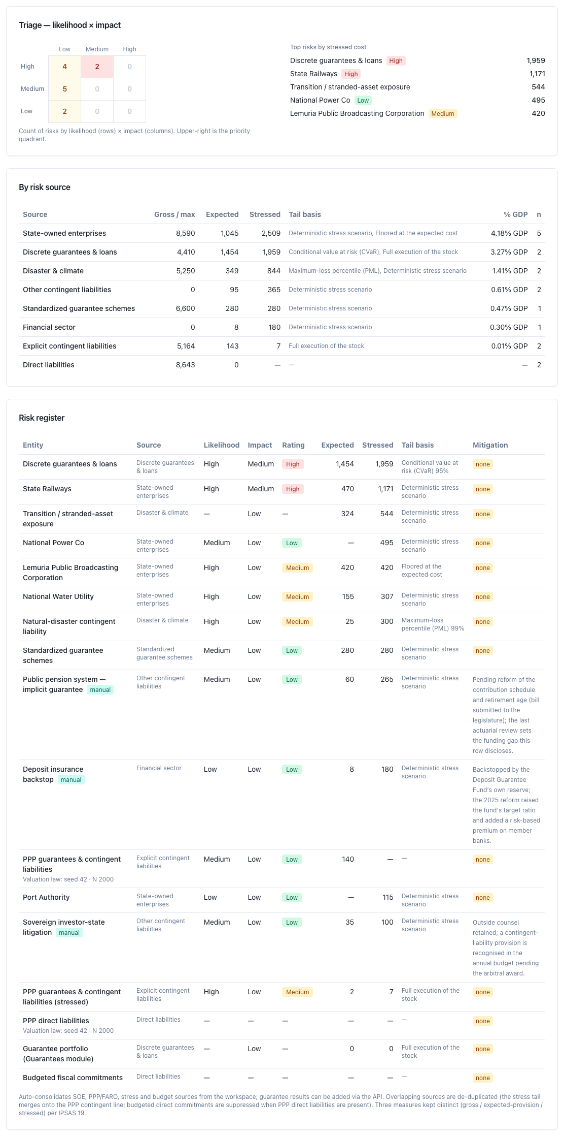
Figure 5.2 — The rest of the cover page, in one run: the 3 × 3 triage matrix (4 · 2 · 0 / 5 · 0 · 0 / 2 · 0 · 0 = thirteen rated rows), the five largest risks by stressed cost with their colour badge, the table by source —with the basis‑of‑tail column and the dash in the stressed subtotal for direct liabilities, which publish no tail— and the row‑by‑row register, with the manual badge on the three hand‑written rows and the amber none badge on the fourteen with no management action. (5.1; Steps 4, 5 and 6.) [note three things, all three limits of this figure: the matrix does not say how many rows it leaves out —four of seventeen, and among them the largest gross exposure in the register—; the register has no gross exposure column, so the two direct rows read as a line of dashes; and the footer has been left behind —it says that budgeted commitments “are suppressed” when they are netted, and that guarantee results “can be added via the API” when the workspace's book enters by default. And one correction to this manual's draft: no row carries the “Undeclared basis” badge today, because the register's fourteen tails all publish their law; the badge exists and this register does not exercise it.]

Basis of the stressed total and correlated portfolio tail — Step 6

Route: the same cover page, two cards under the header. It is the surface that answers the step where the manual takes a side, and it deserves a figure of its own.

The Basis of the stressed total card prints the complete legend of Step 6.3 —drafted by the engine from the actual composition, not a template— and beneath it a table: Basis of the tail · Confidence · Rows · Subtotal · Share of the stressed total. The legend says, in as many sentences as it takes, how many different laws compose the total; that the sum is the sum of the adverse scenarios declared by each family, that it is not a modelled portfolio tail and that it is not an upper bound on anything, with the count of how many of the tails added carry no quantile at all —which is what makes the assertion verifiable—; which confidence levels coexist or that there is none; the reading by law —the expected shortfall rows add to a genuine bound by subadditivity, the quantile rows only under the declared assumption, the deterministic scenario and full call ones carry no confidence—; and, at the end, which contingent rows fall outside the total and with what gross exposure, which is point 5 of Step 6.3.

The card also carries a short line labelled "what this total is", which is where the conditional label of the header lives, and a help text that closes the sentence from the other side: when all the rows share one coherent law at one same level, the legend says so and the sum is a genuine upper bound. It is the only honest way of publishing a label that depends on the composition: making it depend on the composition.

The Correlated portfolio tail card publishes the number of 6.4 alongside the additive one and never in its place: the correlated expected shortfall at the declared level, the same tail assuming independence, the correlation premium —the difference between the two, which is what makes visible why the exercise matters—, the sum of individual tails (comonotonic), the diversification credit and the full call on all the families at once. Beneath, the five largest contributors by component with their share; and at the foot, in small print, the coverage and the assumption: n contingent rows, number of simulations, seed, and the declared correlation matrix with its intra‑family and cross‑family correlation. The two caveats of 6.4 are therefore printed where the reader sees the number.

One note on order and one on language, both verified in figure 5.3. The on‑screen order is basis of the stressed total → non‑duplication → correlated tail, not this text's. And the prose the engine writes on the three cards comes out in English in a Spanish session: the full legend of Step 6.3, the non‑duplication rule of section 2.8 and the names of the four seams. What is translated is the frame —each card's label, its table headers, the basis‑of‑tail vocabulary, the four verdicts and the “what this total is” line—, so that the Spanish reader sees the label in their language and its grounding in another [to be corrected].

Limit. The coverage is reported in rows, not in amount: the reader sees that the number covers n of the register's rows —today 12 of 17—, not what fraction of the exposure they represent. It is one line of calculation and it is worth asking for [to be built].

Non‑duplication between families — Step 4, published as a verdict

Route: the same cover page, a third card. It is the surface that turns the rule of §2.8 into something the reader can check, and it arrived with the eighth collector.

The card first asserts the rule —who the system of record is for each instrument— and then publishes three figures from the guarantee book of every origin: how much maximum exposure it adds, how much was netted off the public corporation rows against it, and the net movement of the two. Beneath, a table with one row per seam and three columns: seam · verdict · amount netted.

The verdicts are four and the vocabulary matters: disjoint perimeters, verified; overlap netted, residual published; not applicable, where one of the two sides is missing; and unverified — may duplicate, which is printed in red. That fourth one is what gives value to the other three: a statement that does not distinguish "I checked that they do not overlap" from "I did not check" is asserting the former by omission, which is exactly the silence Step 4 exists to break. And where the guarantee book is not consolidated in the vintage, the card says so in amber in so many words: guarantees to public corporations, to subnational governments and to credit portfolios are not in any total on that screen.

The same information travels to the document as subsection 2.3.

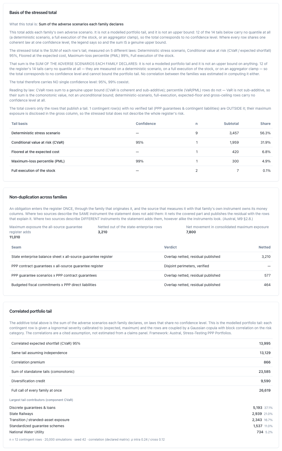
Figure 5.3 — The total, its law and the proof that it is not counting the same thing twice, in a single figure because on the cover page they run consecutively. Basis of the stressed total: the legend says that the total sums tails on five laws, that 12 of the 14 carry no quantile at all, that 95% and 99% coexist, and that one contingent row with no verified tail is left outside with its maximum exposure in the gross column; beneath it, the table by law —deterministic scenario 3,457 (56.3%), CVaR 95 1,959 (31.9%), floored at expected 420, PML 99 300, full execution 7—. Non‑duplication between families: the all‑source guarantee register adds 11,010, 3,210 is netted against the public corporation rows and the net movement is 7,800, with the four seams and their verdict —three “overlap netted, residual published” and one “perimeters disjoint, verified”—. Correlated portfolio tail: expected shortfall at 95% 13,995 against 13,129 under independence, correlation premium 866, comonotonic 23,585, diversification credit 9,590 and simultaneous full execution 26,619, with the five largest contributors and the coverage footer —12 contingent rows, 20,000 simulations, seed 42, ρ within 0.24 / across 0.12—. (5.1; Steps 4 and 6.) [note: the prose of the three cards is in English; the frame is in the session's language. The fifth seam —accounting ↔ risk— does not appear in the table: with its switch off the row is not printed as “not applicable”, it is simply absent, so the reader counts four seams where the method declares five.]

The GDP field and the consolidation notes — Steps 3 and 4

Route: the same cover page, header and band of notes. It is the capture that teaches Step 3 and the seams of Step 4 at the same time, and that is why it is worth a figure of its own even though it is not a screen of its own.

The GDP comes in from a single source: the workspace's macro setting —the same value every other tool on the platform uses—, with per‑query override from the header field. The field comes in empty, and its help text shows the workspace's value: empty means "use the workspace's", not "use zero" nor "use a default value". And the base is printed in the document as a grey note: GDP base: workspace macro setting = value. It is one of the few things the module does better than usual practice, and it is worth saying: rule (a) and rule (b) of Step 3 are executed at a single point and published.

With no GDP configured, the percentages are omitted and the document issues a warning saying so — rule (c) of Step 3, which is the one that prevents publishing "0 % of GDP" for want of a datum.

The consolidation notes are, read in order, the whole of Step 4: how much was netted in each seam, against which rows, with which convention —by period or scalar—, which one was left unnetted and why, and what residual survived. Each note carries its amount.

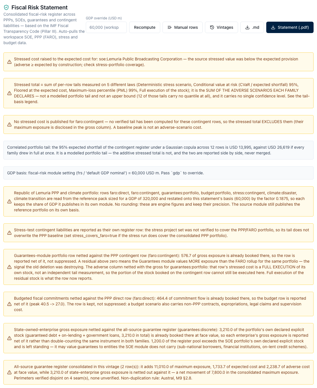
Figure 5.4 — Step 3 and Step 4, at the very top. The GDP override field opens empty —empty means “use the workspace's”, not zero— and the first grey note prints the basis that was used and who resolved it: «GDP basis: fiscal‑risk module setting (frs / 'default GDP nominal') = 60,000 USD m». The eleven notes are Step 4 read in order: the invariant adjustment on one row, the legend of the adverse total, the contingent row left outside, the correlated tail, the GDP basis, the restatement of the Lemuria portfolio by the factor 0.1875, the unverified coverage of the stress run and the three nettings with their amount and the rows that explain them (577 · 464 · 3,210), plus the contribution of the guarantee book. The cover page's four buttons are Manual rows, Vintages, .md and Statement (.pdf). (5.1; Steps 3 and 4.) [note two things: the eleven notes come out in English even when the session is in Spanish —the screen's query does not pass the language; in the exported document all eleven come out in Spanish—; and the field label carries the currency written by hand (USD m) instead of the workspace's. A third thing, which belongs to the run and not to the product: this figure was taken before the production deployment of midday on 2026‑09‑28, and since that deployment the same screen also prints, above the GDP field, a provenance warning —«One or more FARO projects were calculated with an earlier engine build»— which figures 5.9 and 5.11, taken afterwards, do carry. It moves no figure: it is the guard that says a "Calculate All" on the contract portfolio would refresh the cached results. In the exported document it appears as a twelfth note, after the eleven of method.]

Manual rows — Steps 4 and 8

Route: …/frs/manual-rows, from the Manual rows button on the cover page. Input: whatever the analyst writes. Output: register rows marked as manual. What the analyst decides: everything, and signed.

It is the editor for the risks no engine produces. Each row carries: the entity's name, the family, a description, the three monetary measures, the probability, the measurement basis or standard, the mark of provision recognised versus merely disclosed, the mitigation action —with a help text that says exactly where it will appear: in the mitigation actions section of the statement— and the supporting documents, which are attached by reference with their label and distinguish whether they are an assessment of a discrete guarantee, of a standardised scheme, or any other document.

Two disciplines of Step 4 are executed here and are worth pointing out: manual rows pass through the same deduplication point as the engine ones, so that two manual rows with the same identifier are merged instead of duplicated; and the identifier prefixes of the automatic sources are reserved and a manual row that tries to use them is rejected with its explanation, in the editor and also in the programming interface. The screen's footer says both things, and it also says that the amounts are in the workspace's currency, in millions — the only place in the module where the unit is written.

Demonstration seed. The module seeds three disclosed rows with their management action: a pending investor‑State arbitration over a terminated concession, with a budget provision and external counsel retained; the backing of the deposit guarantee fund, with the reform that raised its target ratio and added a risk premium; and the implicit guarantee of the defined‑benefit pension system, with the reform of the contribution schedule and of the retirement age in progress. They are the three families §2.3 shows among the most expensive and that no portfolio engine produces. The seeding is additive: it touches no row the analyst has written, and the reset deletes only its own three.

Limits. (i) The form has no law‑of‑the‑tail field. The programming interface accepts it and validates it against the closed vocabulary of Step 2.3; the screen does not offer it, so that every tail written from the editor arrives with no law and the register reports it —correctly— as Undeclared basis. It is the only place in the product where the discipline the module imposes on the engines cannot be met from its own screen [to be built]. (ii) Writing requires a licensed workspace, not merely an account. The previous footing said “a guest gets a 403”; the figures session measured it precisely and the subject of the 403 is not the user but the workspace: a workspace created today is born on the guest plan, and the guest plan returns guest_action_blocked on every save —including for a registered account that owns the workspace—. Reading does not. It is the same door that closes the module's four downloads (5.10).

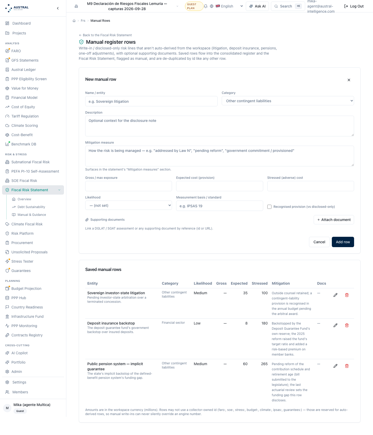
Figure 5.5 — The editor for the risks no engine produces. The form asks for name / entity, category, description, mitigation action —with the help text that says where it will appear: «Surfaces in the statement's “Mitigation measures” section»—, the three monetary measures, the likelihood, the measurement basis / standard, the recognised provision (vs disclosed‑only) mark and the supporting documents, which are attached by reference. Beneath it, the three seeded rows —investor‑state litigation 35 / 100, deposit insurance 8 / 180 and the pension system 60 / 265— each with its declared management action. The footer states the two Step 4 disciplines: amounts are in the workspace currency, in millions —the only place in the module where the unit is written— and the identifier prefixes of the automatic sources are reserved. (5.1; Steps 4 and 8.) [note: there is no law‑of‑the‑tail field —the form's ten fields are all in view and none is it—, so every tail written from here arrives with no law.]

Vintages — Step 9

Route: …/frs/vintages, from the Versions button on the cover page — the label 5.5 declares as a deliberate divergence. Input: a name and a cut‑off tag. Output: the frozen statement, and the comparison.

The screen does two things. It freezes the statement of the moment with its complete scope —which collectors entered, which GDP, which currency— and saves it with its name, its cut‑off tag and its summary of headlines. And it compares: one vintage is chosen as the baseline and another vintage, or the live statement, as the term of comparison, and the screen delivers the movement line by line —Register line · Change · Δ gross · Δ expected · Δ adverse scenario · Δ realised— classified into addition, removal, modified or unchanged, plus the variation of the totals.

That last column is new and it closes a gap this manual had noted: the realised cost is now attributed to the row that generated it and not only to the total. It was the cause Step 9.3 names as the most important to explain —what the State actually paid— and it was the only one of the five the comparison could not locate. The screen's footer says, with the four columns in view, that the four measures are not added to one another.

Two rules of Step 9 are executed and deserve to be stated. The first: the vintage saves the statement produced, not the inputs, so that a later change of engine cannot move a figure already presented — which is the whole of rule 9.1. The second: when a vintage is compared against the live statement, the live statement is reconstructed over the same scope with which the vintage was frozen, not over today's scope — which is rule 9.2, and it is the one that prevents switching on a new collector from appearing as a deterioration in the country's risk. The screen also warns when the two vintages are in different currencies and the variations mix units.

Limits. (i) Freezing a vintage requires a licensed workspace. The screen offers the save block and the summary line for the live statement, and the Freeze current statement button returns guest_action_blocked on a workspace on the guest plan — which is the plan a workspace created today is born on. With the workspace on the ministry plan the button answers, and that is what figure 5.6 shows: the frozen vintage and the comparison against the live statement. The limit belongs to the product, not to the figure, and it is worth reading alongside Step 9: the trial without registering reaches as far as reading the statement and stops just short of publishing it. (ii) The attribution by cause of Step 9.3 does not exist. The screen distinguishes an addition from a removal and from a modification; it does not distinguish a change of measurement from a change of risk, which is the distinction that makes the comparison useful. The analyst writes it over the list of movements, and it is half an hour's work a year [to be built].

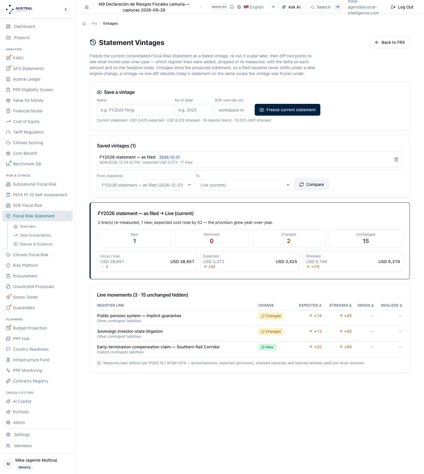
Figure 5.6 — The whole of Step 9, from the rule to the movement. The description prints rules 9.1 and 9.2 where the analyst reads them: «vintages store the statement as produced, so a presented baseline is never altered by a later engine change; a vintage‑vs‑live comparison rebuilds today's statement on the same scope the vintage was frozen with». At the top, the save block —name, as‑of label and alternative GDP— with the status line of the live statement. In the middle, the vintage frozen in this run: «FY2026 statement — as filed», as of 2026‑12‑31, over the seventeen‑row register of section 4. Below, the comparison against the live statement: 1 new · 0 removed · 2 changed · 15 unchanged, the three headline totals with their movement —gross 38,657 → 38,657 (0), expected 3,373 → 3,425 (+52), stressed 6,144 → 6,319 (+175)— and the movements table with its four delta columns, one per measure, each line's badge, and the dash where the measure did not move, which is the rule of the four distinct measures exercised inside the comparison itself. (5.1; Step 9.) [note three things. The first is how the movement was produced, and it is declared because it belongs to this run and not to section 4: the vintage was frozen over the seventeen‑row register and then two manual rows were re‑measured and a third was written, as an analyst would a year later; once the figure was taken the movement was undone and the register returned exactly to its seventeen rows and its four headline totals —the same thing figure 5.7 does with its six assumptions and 5.13 with its three rules—. The second: the comparison does not tell a re‑measurement from a change of risk (limit (ii)); the two re‑measured rows and the new one carry the same class of badge a real deterioration would carry. The third belongs to language and to this screen: over a Spanish session, the saved vintage's line says «expected» and «lines», the target of the comparison is labelled «Live (current)» and the movement's headline sentence comes out wholly in English —«2 line(s) re-measured, 1 new; expected cost rose by 52»—; the product writes all three, not the demonstration pack, and the first two are in the screen, not in the engine [to be corrected].]

Debt sustainability — bridge to Pillar III

Route: …/frs/dsa. Input: six typed fields. Output: the debt‑to‑GDP path and a debt transparency score.

It is taught once, and it is taught declaring what it is. The screen projects the debt‑to‑GDP path from six assumptions the analyst writes —initial debt, real rate, real growth, primary balance, horizon and maturing debt—, and delivers terminal debt, the debt‑stabilising primary balance and a risk signal with its year‑by‑year path; and separately it scores debt transparency from four questions and a publication lag.

The limit is the point of the screen, and it has to be written in so many words: it does not read the register. Neither the stressed cost, nor the gross exposure, nor what was realised in the period enters the path; the six assumptions are the analyst's and none comes from the consolidation. And the transparency score asks the analyst whether the debt of public corporations is disclosed, in a workspace where the platform has the module that calculates it. Pillar III places long‑term sustainability alongside the register of specific risks because they are the same conversation; here they are on the same screen and they do not talk to each other [to be built].

It is, for that reason, exactly the scope §1.1 declares: the statement names sustainability analysis, says what the crossing would be that belongs to it —the realisation of the register as a shock to the path— and declares that today it is not done. Describing it otherwise would be promising an integration that does not exist.

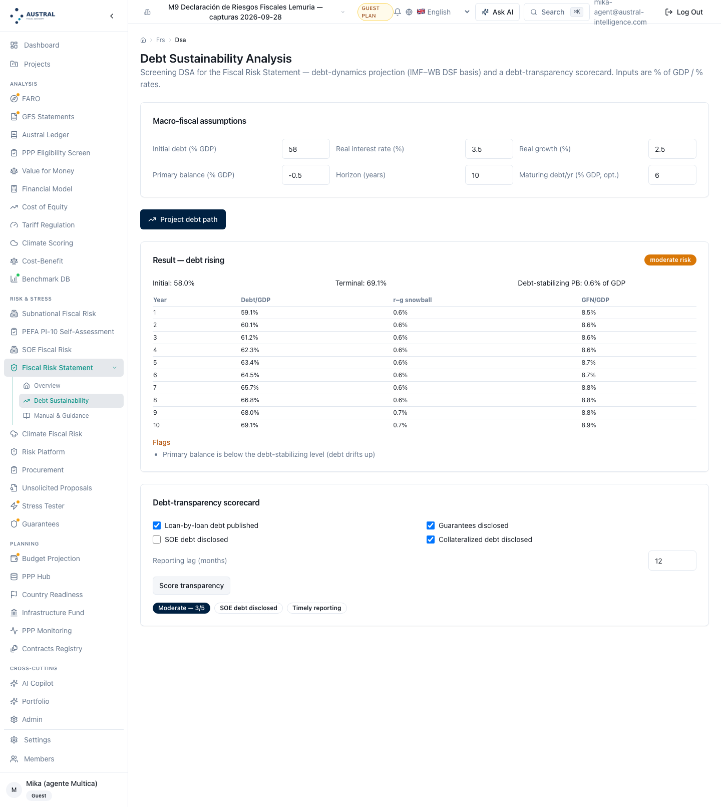
Figure 5.7 — The whole screen, and the limit is visible in it without needing explanation: the six assumptions are typed —initial debt 58.0% of GDP, real rate 3.5%, real growth 2.5%, primary balance −0.5%, horizon 10 years, maturing debt 6.0%— and none comes from the register. The projection returns debt rising · moderate risk, terminal 69.1% of GDP and a debt‑stabilising primary balance of 0.6% of GDP, with the year‑by‑year path and the r−g snowball. Beneath it, the transparency scorecard: four checkboxes and a reporting lag, returning Moderate — 3/5 and naming the two gaps —SOE debt disclosed and timely reporting—. (5.1; bridge to Pillar III.) [note: the six assumptions are the analyst's and are declared as assumptions of this figure, not measured; section 4 does not fix them. The question «is the public corporations' debt disclosed?» is put to the analyst in a workspace where the module that calculates it carries five enterprises.]

On‑screen manual — orientation

Route: …/frs/manual, in Spanish and in English. It is the summary of the method inside the product: what it consolidates, the method, the thresholds and ratings with the three‑by‑three matrix printed, the three‑row worked example and the references. The three‑row example is pinned to the engine by a test: if a threshold or the matrix changes, the test fails and the page has to be updated in the same change. It is the reason why §4.2 can use that same minimal example as an arithmetic box with no risk of its going out of sync.

Limit. The on‑screen manual has been left behind on the seams and it has to be corrected before the capture. It asserts that budgeted direct commitments "are suppressed" where the contract portfolio already reserves a direct row —today they are netted by period and the row survives with its residual—; it does not mention the guarantees ↔ contracts seam, which is the one that moves the register most; it does not mention the public corporations ↔ guarantee book seam, which is the most recent; and it mentions none of the four surfaces that arrived later —the manual rows editor, the vintages, the register workbook and the accounting note— nor the discipline of the law of the tail, which is the module's most important change. And one line more, which the figures session added: it says the GDP basis is “the workspace's macro GDP (Macro / ‘GDP Nominal’)”, when the module resolves its own setting first —which is what the note in figure 5.4 prints— and only falls back to the macro if it has none [to be corrected]. The series' commitment stands: the on‑screen manual is aligned with this manual once this manual is written, as was done with the modules of wave 1 (5.8).

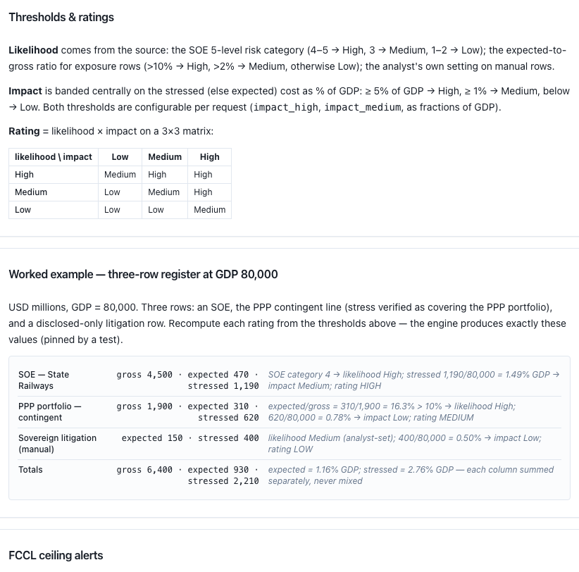
Figure 5.8 — The method inside the product. Thresholds & ratings: likelihood comes from the source —the public corporation's risk category, the expected‑to‑gross ratio, or the analyst's own setting on manual rows—, impact is banded centrally over the stressed cost as a % of GDP (≥ 5% high, ≥ 1% medium) and both cut‑offs are configurable per request; beneath it, the 3 × 3 matrix printed. And the worked example of three rows at GDP 80,000, with the arithmetic of each rating written alongside — the same example section 4.2 uses as its arithmetic box, and which a platform test keeps pinned to the engine. (5.1; Steps 5 and 6.) [note: this figure is the English edition of the on‑screen manual; the Spanish edition of this manual carries the Spanish one, framed identically. The module serves both from one page.]

The statement in markdown and in PDF — Step 9, the deliverable

Route: the two download buttons on the cover page — .md and Statement (.pdf). Both pass the session's language and the substitute GDP if there is one.

The two documents today have the same sections, in the same order, with the same titles, and that is a recent change worth pointing out because it affects what section 4 numbers: until recently the PDF —which is the main button— carried three sections and the markdown six, so that whoever opened the PDF never saw the risk register nor the mitigation actions, which are the two pieces Pillar III asks for most explicitly. Today the section titles come from a single shared definition and a parity test sustains that they cannot diverge again.

There are six sections, plus three subsections:

1. Executive summary — the four figures, the correlated expected shortfall if it is available, the distribution by rating, and the stressed total with its qualifier on the same line.
2. Consolidated summary — the table by family, with the basis‑of‑the‑tail column and the dash instead of the zero where the family publishes no tail. 2.1 Basis of the stressed total — the legend of Step 6.3 and the table by law. 2.2 Correlated portfolio tail — the number of 6.4 with its contributors and its footnote on coverage and matrix. 2.3 Non‑duplication between families — the rule of §2.8 with the verdict for each seam and the net contribution of the guarantee book.
3. Specific fiscal risks — the register, one block per family.
4. Probability × impact matrix.
5. Mitigation actions — the table of rows with a declared action and, at the foot, the count: how many of the disclosed risks record an action and how many do not yet. Where none has one, the prose says so explicitly instead of omitting the section.
6. Methodology and basis of preparation — six statements about the document itself, including the two this manual considers non‑negotiable: that every stressed cost carries the law that calculated it and that the total adds laws that do not combine, and that a contingent row with no verified tail leaves the column empty instead of repeating its baseline peak.

It is worth saying, about section 1, that the stressed total comes out with its qualifier on the same line and that that qualifier is today the new label of Step 6. An executive summary is exactly the place where a figure travels alone; here it cannot.

The preamble carries the coverage sentence —risks not listed are not covered by this statement— and the consolidation notes go above, before the executive summary.

Limits. (i) Section 3 has no gross exposure column — the same limit as the cover page, and with the same consequence: direct rows come out as dashes. (ii) The PDF is typeset with a Latin‑1 repertoire font: it keeps accents and ñ, so that the statement in Spanish no longer prints "Declaracion", but it substitutes the characters outside that repertoire —the em dash, typographic quotation marks, the greater‑than‑or‑equal sign and the multiplication sign— with typewriter equivalents. It is acceptable in a working document and a Unicode font is advisable before the PDF becomes a ministry's deliverable [to be corrected]. (iii) All eleven consolidation notes now reach the three exported documents in Spanish. This edition of the manual declared nine of eleven —the two the eighth collector brought after the translation were missing—; the measurement of 2026‑09‑28 over production gives zero of eleven untranslated, and a test that walks the live output of the complete register closes the whole class of defect rather than its instances. What stays open is the other half, and it is the one the reader sees: the screen still shows them in English, because the query that feeds it does not pass the language (figure 5.4) [to be corrected]. (iv) All seventeen row names now come out in Spanish, and one leak remains. The product's two tables of names —the labels the adapters invent and the names the demonstration pack itself wrote, kept separate on purpose because a name a user types is data and is never translated— went to nine and nine entries and today cover seventeen of seventeen: the exception this edition declared —the book of one‑off guarantees— now has a label. The leak stands, and its single cause can now be named: eight English names appear all the same in the Spanish document, not in the register's column but inside the legend of the tail, which quotes the source name instead of the translated label. Translating the label is not enough if the generated prose quotes the other one [to be corrected]. And there is a third half to this same matter, the worst of the three because it is what the reader sees first: the screen followed neither table (limit (v) of the cover page).

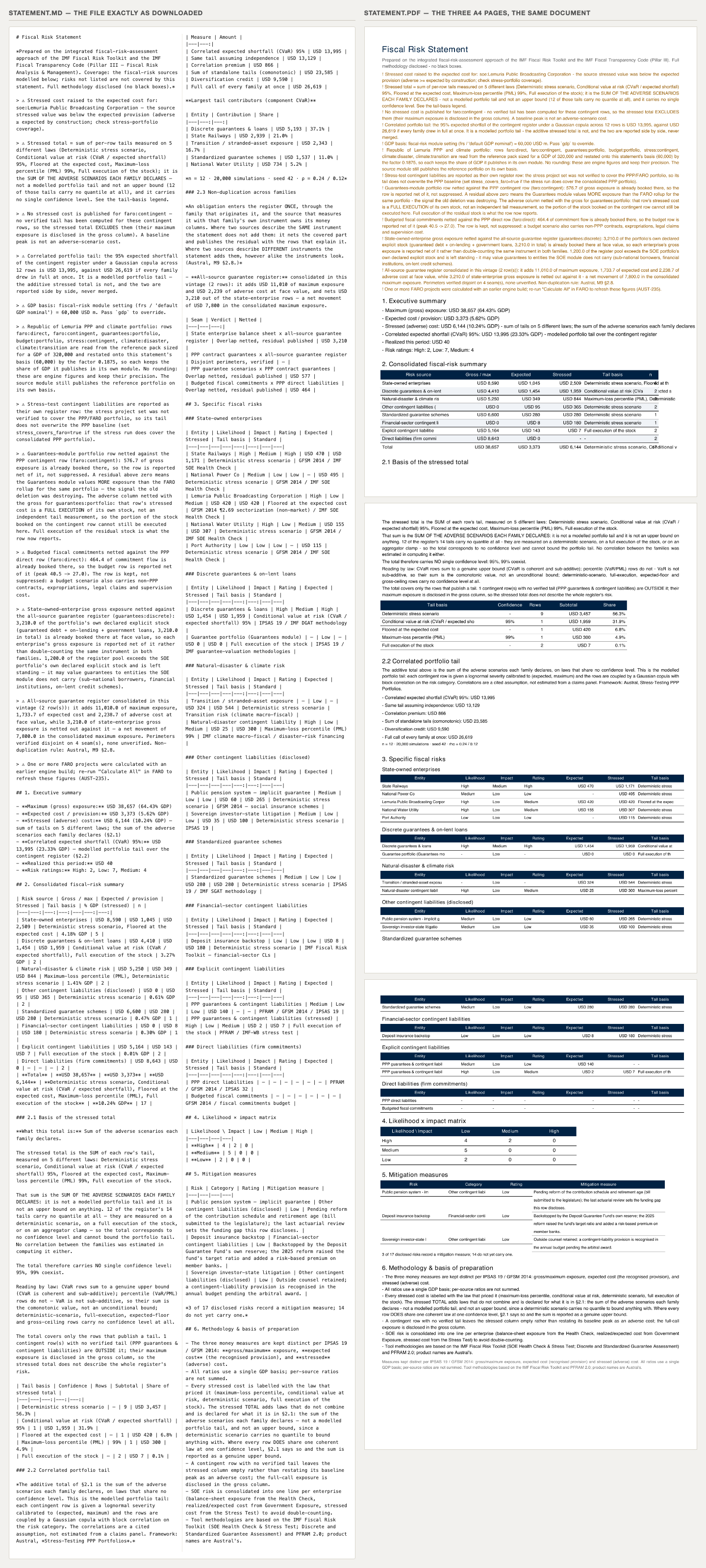
Figure 5.9 — The two deliverables of the cover page's .md and Statement (.pdf) buttons, side by side and whole: on the left the markdown file exactly as it downloads, on the right the PDF's three A4 pages. The same six sections, in the same order, with the coverage preamble and the consolidation notes at the top, before the executive summary, and the executive summary opening with the four figures of 4.3 —38,657 · 3,373 · 6,144 · 40— and the adverse total carrying its qualifier on the same line. (5.1; Steps 4 to 9.) [note two things, and both belong to the PDF, not to the markdown. The first is about language and it contradicts the claim that the three exported documents arrive wholly in Spanish: the eleven notes of method do come out in Spanish in both formats, but the PDF prints its own frame in English —the preamble and coverage paragraph, the two qualifiers of the executive summary (the one on the stressed total and the one on the correlated tail) and the document's footer line—, all of which the markdown carries in Spanish. The same document, asked for in the same language, does not come back with the same translation depending on the format [to be corrected]. The second is about typesetting and is plain to see in the section 2 table: the columns are fixed‑width, so long family names are cut mid‑word —«Garantías discretas y préstamo», «Otros pasivos contingentes (di»— and the tail‑basis column overflows past the right margin; Spanish suffers more than English because its labels are longer, but the defect is in both [to be corrected].]

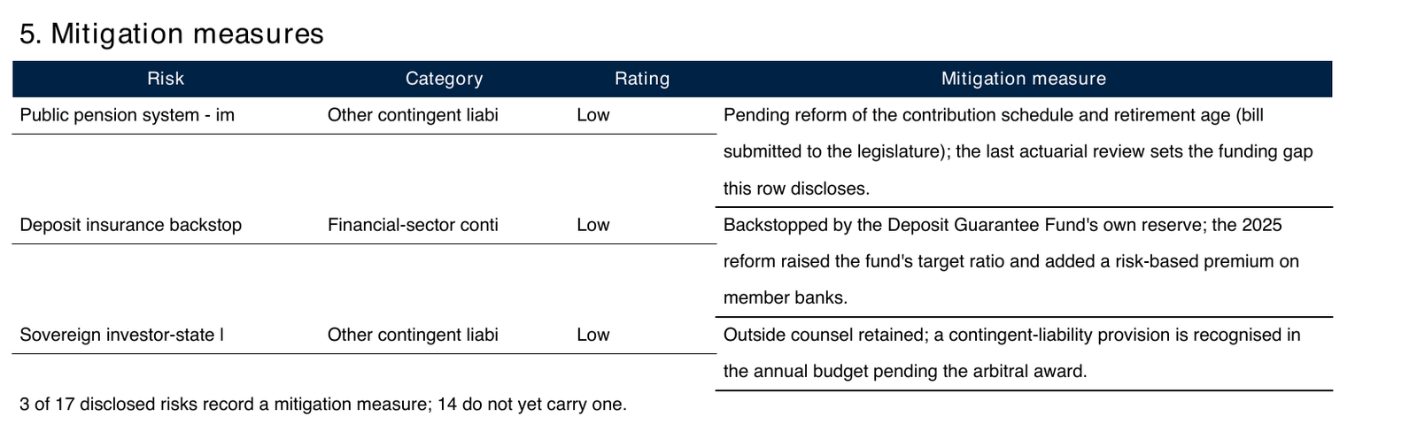
Figure 5.10 — Section 5 of the document, up close. The table carries the three hand‑written rows with their category, their rating and the mitigation measure declared, and at the foot the count the method asks for: «3 of 17 disclosed risks record a mitigation measure; 14 do not yet carry one». It is the section that turns a register into a statement: it says how much of the country's risk has an owner and how much does not. (5.1; Steps 4 and 8.) [note two things. The three row names come out translated in the Spanish edition —«Sistema público de pensiones», «Respaldo del seguro de depósitos», «Litigio inversionista‑Estado»—, which is the demonstration pack's name table working in the document and not on the screen (figure 5.5); but the text of the mitigation measure stays in English, because it is data the pack wrote and data is never translated. And the fixed column width cuts again: «Public pension system - im», «Other contingent liabi». All three are rated Low, consistent with the matrix of 4.2: low impact and medium or low likelihood.]

The register workbook — audit of section 6

Route: a download by call; it has no button on the screen [to be built]. It is the format in which a fiscal risk unit really works the figures, and it has three sheets:

• Register — one row per obligation, with thirteen columns: source, entity, family, gross exposure, expected cost, stressed cost, basis of the tail, confidence, % of GDP (expected), probability, impact, rating and standard, with the rating shaded and a total row. It is the only surface of the product that carries gross exposure and rating in the same table, and that is why it is the one that makes up for the cover page's limit.
• By family — the subtotals with their laws of the tail.
• Summary — the four headlines, the two percentages of GDP, the complete legend of the stressed total with its table by law, and the matrix.

Plus a bases of preparation sheet with the document's three methodological notes.

Limit. The three notes of the bases sheet are not in the module's translation table: in a workbook requested in Spanish, that sheet falls back to English through the fallback mechanism. It is a minor consequence of the language and it is the sheet an auditor reads first [to be corrected].

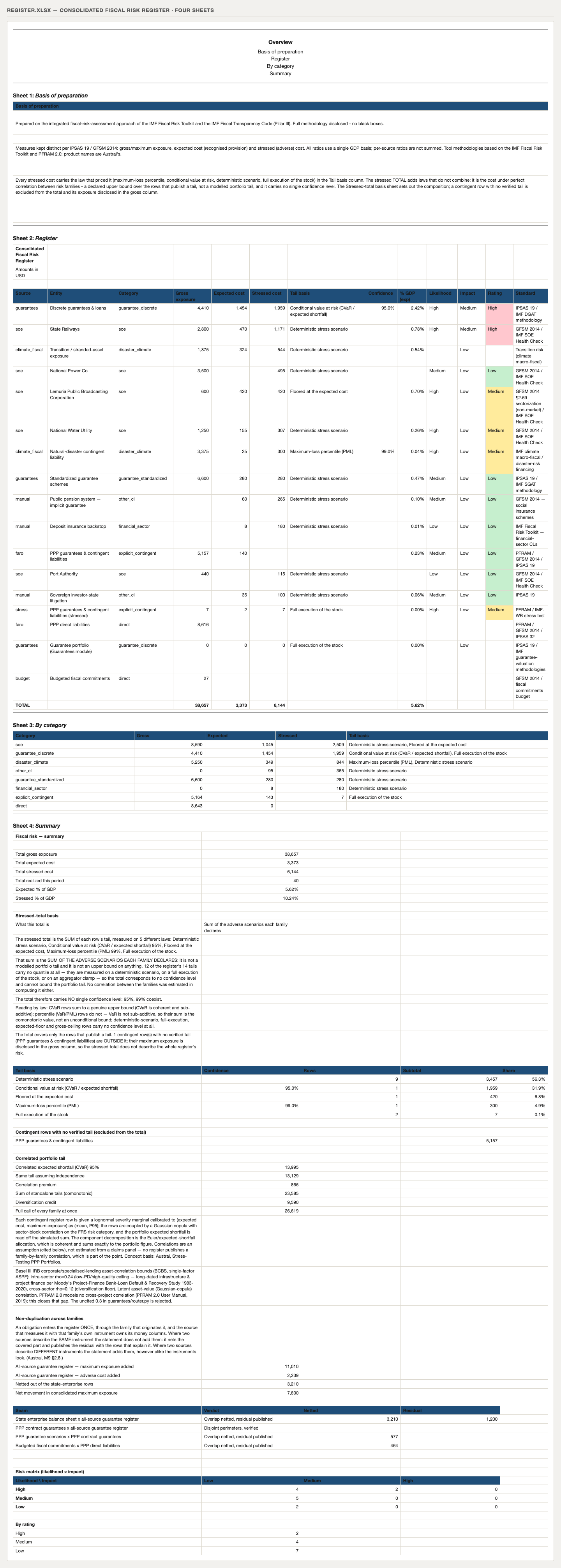
Figure 5.11 — The whole workbook, its four sheets in sequence. Basis of preparation opens with the document's notes of method. Register carries the seventeen rows with their thirteen columns and the total row —38,657 · 3,373 · 6,144 · 5.62% of GDP, section 4.3 exactly—, with the rating shaded and, above all, with the gross exposure column next to the rating: it is the only surface of the product that has them together, and that is why it fills limit (ii) of the cover page — the two direct rows, which on screen read as dashes, publish their 8,616 and 27 here. By category gives the eight subtotals with their law of the tail. Summary closes with the four headline figures, the two percentages of GDP, the full legend of the stressed total with its table by law (3,457 · 1,959 · 420 · 300 · 7), the correlated tail (13,995 · 13,129 · premium 866 · comonotonic 23,585 · diversification 9,590 · full execution 26,619), the four non‑duplication seams with their verdict and their netting (3,210 · 577 · 464, net movement 7,800) and the matrix. (5.1; Step 6 and section 6.) [note three things. The subtotals sheet is labelled «By category», not «By family» as the prose above names it. The language limit this manual declares is confirmed and widened: the basis of preparation sheet falls wholly to English, and to it is added the paragraph explaining the copula and the calibration inside the summary sheet, which is the workbook's other block of generated prose; everything else —sheet names, headers, the seventeen entities, the tail bases, the seam verdicts— comes out in Spanish [to be corrected]. And the workbook still has no button: it is asked for by call.]

The sovereign note on provisions and contingent liabilities — Step 7

Route: three calls —data structure, workbook and A4 document—; it has no screen [to be built]. It is, together with the statement, the manual's second deliverable, and it is the one an accountant general presents.

The note decides recognition row by row, which is the substantive change to this surface. Each non‑direct row passes through the three conditions of ¶22 —present obligation, probable outflow, reliable measurement— assessed one by one and with three verdicts: met, failed and undetermined. A row is recognised only with all three "met"; an undetermined never recognises. And the note publishes, per row, which condition stopped it and on what basis the obligation arose, so that the border between recognising and disclosing is traced by the standard and not by the collector that wrote the row.

It also publishes the measurement standard of each amount: the recognised total comes out broken down between expected credit losses of the financial instruments standard and the best estimate of ¶44 of the provisions standard, with the explicit statement that there is more than one standard where there is — because two amounts measured under different standards are not a single figure (§2.5). The vocabulary of standards has four values and two of them are not accounting measurements: the statistical measure of the national accounts book and the screening model estimate. A row measured that way returns undetermined on ¶22(c), not "failed": the defect is the absence of an accounting measurement, not an unreliable number.

And it applies the remote possibility cut‑off of ¶36, with the same single value the accounting note of the guarantees module uses —5 %, on the ratio of expected cost to maximum exposure— published alongside the note with its criterion and with the statement that the standard fixes no figure. The presentation is flag and do not withdraw: the remote row is disclosed anyway, with its flag and with the separate subtotal a preparer needs in order to exercise —or not— the dispensation. Rows that cannot be assessed against the cut‑off are counted as such and are never presumed remote.

The rest stands as it was: it splits the register into provisions recognised —at present value— and contingent liabilities disclosed —with their maximum exposure and their estimated financial effect where there is one—, aggregates by currency and by family without adding across currencies and flags where there is more than one, counts the reclassified rows with their reason, and excludes the direct rows counting them separately because they are a recognised liability under the concessions standard and go to the balance sheet. The workbook has five sheets: provisions recognised, contingencies disclosed, by currency, by family and the general government narrative.

Limits. (i) It has no screen: it is reached by call or by export [to be built]. (ii) The reconciliation of Step 7.2 is not issued as a table in the note: the counts all exist —recognised by standard, reclassified, direct excluded, contingencies disclosed, and the distribution of conditions that stopped each row— and the analyst arranges them into the lines of the bridge [to be built]. (iii) The note today recognises only the two rows of the guarantee families, and that is no longer an artefact of the split but a result of the test: the contract, public corporation, climate and stress rows have no present obligation identified by instrument, or their amount is not an accounting measurement. The difference from the previous edition of this manual is that now it is written which of the two things happens in each row, and a preparer can disagree with one in particular.

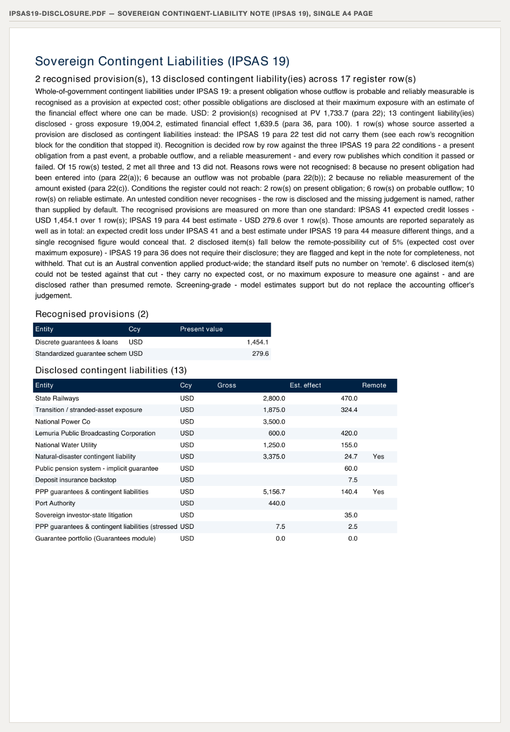
Figure 5.12 — The note, on a single A4 page. The headline counts the perimeter —2 provisions recognised and 13 contingent liabilities disclosed across 17 register rows— and the general‑government narrative publishes, in one paragraph, everything section 7 of the method requires: the total recognised at present value 1,733.7 of para 22, the gross exposure disclosed 19,004.2 and its estimated financial effect 1,639.5 of para 36 and para 100, the reclassified row with its reason, the distribution of the conditions that stopped each row (8 with no present obligation, 6 with no probable outflow, 2 with no reliable measurement; 2, 6 and 10 that could not be tested), the breakdown of the recognised total by standard —1,454.1 of expected credit loss and 279.6 of para 44 best estimate— and the 5% remote‑possibility cut with its 2 items flagged and not withdrawn and its 6 that could not be tested. Below, the two tables: provisions recognised, and contingencies disclosed with their gross exposure, their estimated effect and the remote flag. The figures are those of 4.7, without a single difference. (5.1; Step 7.) [note: the note is the one deliverable that ignores language entirely. Asked for in Spanish and asked for in English it returns the same file byte for byte —verified in both formats—, and Spanish appears nowhere in it: not the title, not the narrative, not the headers, not the names of the thirteen disclosed rows, which the workbook and the statement do translate. It is the costliest language defect this manual declares, because this is the document an accountant general files [to be corrected]. And the fixed width cuts a cell again: «Standardized guarantee schem».]

Ceiling alerts — Step 6, the reading against the ceiling

Route: …/portfolio/alerts. It is named and taught once, as the other end of the register (Austral, The Pipeline Under the Ceiling).

The analyst defines rules —total maximum contingency below an amount, commitments over GDP below a percentage, a single project's contingency, number of high‑risk projects, debt over GDP— with their operator, their threshold and their severity, and the screen evaluates them. Two things are well done and worth saying, the first with more precision than this edition gave it: the percentage‑of‑GDP rules do not merely use “the same workspace GDP”, they use the same resolver as the statement —the module's own setting consulted before the macro—, so that the two surfaces cannot disagree even when the workspace holds both values; and a percentage rule with no GDP configured returns an explicit cannot be evaluated status, never a silent pass.

The limit is important and corrects what might be assumed: the alerts do not read the consolidated register. They re‑aggregate the contracts side on their own account —from the same result cache the portfolio collector uses, so that they agree with those two rows— and they walk the unmodelled rows by a route of their own. Public corporations, climate, the guarantee book and the hand‑written rows do not reach the ceiling. The ceiling is therefore read today against the concessions portfolio and not against the statement, which is the reading Step 6.6 asks for [to be built]. The figure measures it: the maximum‑contingent rule is evaluated over 5,156.7, which is the two contract‑portfolio rows, and not over the register's 38,657.

A second limit, and it is one of language. The alerts screen is not translated: labels, metric names, operators and result messages come out in English in a Spanish session, and only two headers of the rules table —Nombre and Métrica— are in Spanish. It is the only one of the six screens this manual teaches that does not speak the session's language; the other five do, except in the prose the engine writes [to be corrected].

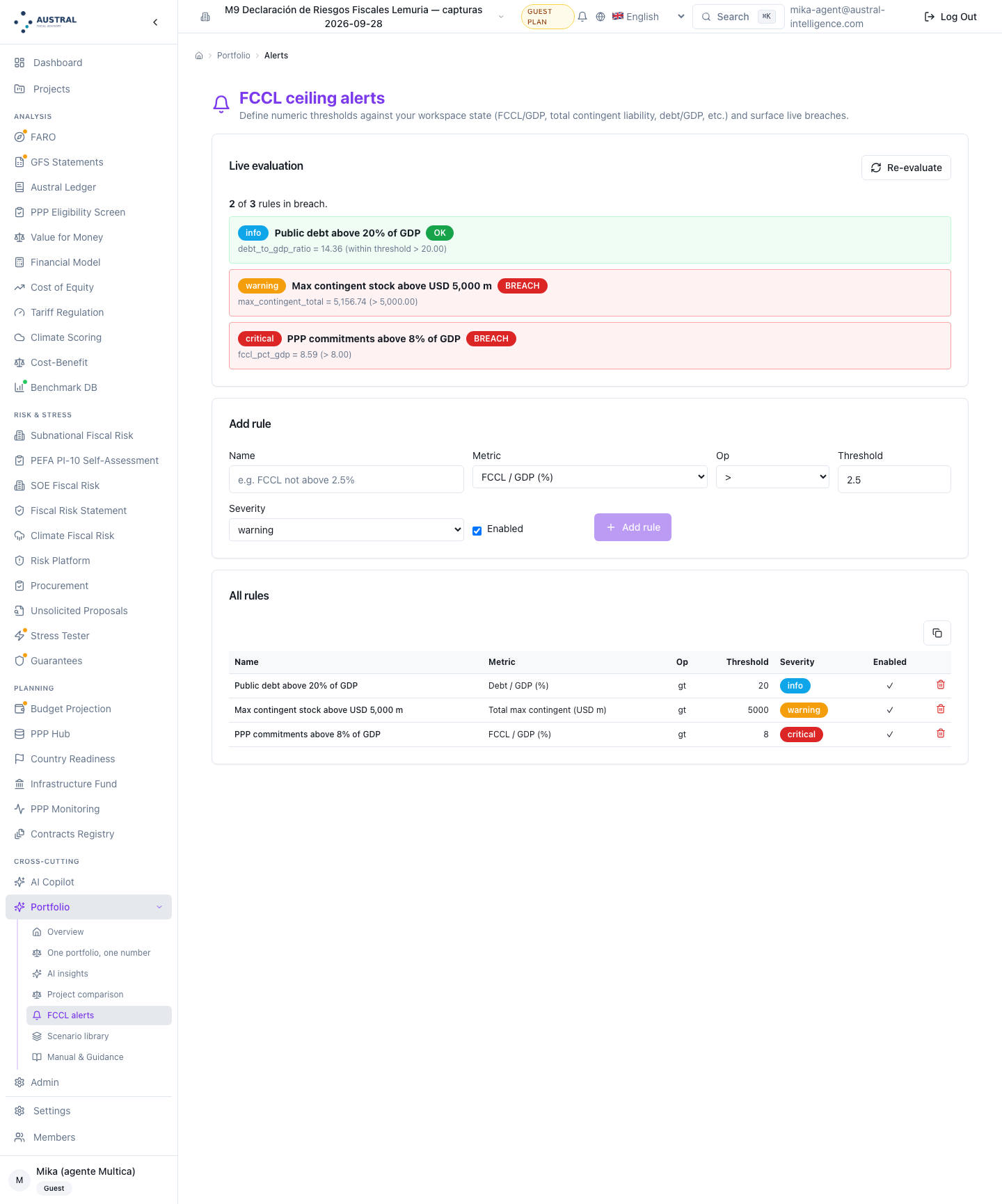
Figure 5.13 — The other end of the register. Three rules defined and evaluated live, 2 of 3 in breach: the maximum contingent stock 5,156.74 > 5,000 (warning), PPP commitments 8.59% > 8% of GDP (critical) and public debt 14.36%, within the 20% threshold (info). The two percentage rules use the same GDP of 60,000 as the statement —the module's own setting, not a second value—: 5,156.74 / 60,000 = 8.59%. Beneath, the add‑rule form with the vocabulary's six metrics and the four operators. (5.1; Step 6.6.) [note two things. The first is the underlying limit and it is visible in the figure: the ceiling is evaluated over 5,156.74 and the consolidated register sums 38,657 — public corporations, climate, the guarantee book and the hand‑written rows do not reach the ceiling. The second: this manual's draft caption asked for «the cannot be evaluated status of a third rule», and it could not be shown: that status requires a workspace with no GDP configured and this workspace has its own, which the other twelve figures depend on. The path exists and is verified in the code; the screen would return it in the same shape as the other two statuses.]

5.2 Where each row comes from

Eight collectors fill the register, plus the manual rows editor. The table says which column each one fills, on what basis, which switch controls it and how it comes by default. It is the best methodological note there is in the product and this manual cites it because it is the table Step 2, rule (c), asks for and that the row model does not yet carry.

Two readings of the table. The first, about the one that comes off: the general ledger is off because its provisions are the accounting view of the same guarantees the contract portfolio already captures, and switching it on duplicates unless the ledger has genuinely distinct items. It is the accounting ↔ risk seam of Step 4.5, and the decision to switch it on belongs to the document's owner.

The second, about the column of bases: five different bases are stacked in the "expected" column —a present value of lifetime credit loss, a peak‑year provision, a net fiscal cost for the financial year, an expected annual loss, an accounting provision— and four different laws in the "stressed" column. The four laws are labelled per row and published in the legend; the five bases are not. That asymmetry is, today, the most quotable gap between section 3 and section 5, and this table is what the analyst uses in the meantime.

5.3 The five seams, in the product

Four precisions the register publishes with every netting and that this manual inherits as a reading rule:

• Only the gross column nets like for like. In the expected one a present value is netted against a peak‑year flow; that residual is indicative. The residual of the gross column is the reliable reconciliation signal.
• A tail is only netted against a tail of the same law and at the same confidence level. Where the laws do not coincide, the tail stands and the register notes which laws there were on each side. It is the rule that prevents a full call from being subtracted from an expected shortfall.
• The public corporations seam is an aggregate netting, not an instrument‑by‑instrument identification, because the guarantee book carries no per‑line link to a specific enterprise. Hence two honest imprecisions the register publishes instead of hiding: a surplus in the book is not assumed to be more public corporation exposure —it may value guarantees to subnational borrowers or to financial institutions that the enterprises module does not carry— and a declared explicit stock that exceeds the book leaves the excess unnetted, as a reconciliation gap.
• No netting deletes a row. The row survives with its residual, and a residual above zero is information: it means that one of the two sources values it higher than the other.

And the limit Step 4.5 anticipates: the switch of the guarantees ↔ contracts seam comes on, and that is correct only if the two sources value the same portfolio. If the workspace's guarantee book covers a set disjoint from the contract portfolio, the netting does not correct a double count: it erases the family. The check is the analyst's, they make it before publishing, and the tool does not make it for them: the switch exists precisely so that it can be turned off in that case.

5.4 What the screen says and what the engine does

Four conventions that have to be declared, with their consequence measured in the example of section 4. All four are different from those a reader of the index would expect, because the ones listed there have already been corrected and it is worth saying which they were: the adverse column of the contracts row no longer repeats its baseline peak —it is left empty—; the stressed total is no longer published without its legend, and that legend no longer promises an upper bound it does not deliver; the PDF no longer has fewer sections than the markdown; no row publishes a tail above its own maximum exposure; the year‑on‑year comparison attributes the realised cost to its row; the accounting note decides ¶22 row by row and applies the remote cut‑off. The ones that remain are these:

1. The on‑screen register has no gross exposure column. The table by family has it, and the register workbook does. The consequence is concrete and appears in the figure: the two direct rows —the largest exposure in the document— read as a line of dashes, and a reader who looks only at the register will conclude that there is nothing there.
2. The figures carry no unit. The header and the tables print the amount with its currency code and without saying that they are millions. The only surface that says so is the footer of the manual rows editor. For a document a minister quotes, the unit is not a typographical detail.
3. The matrix does not say how many rows it leaves out. It counts the rated ones and does not count those that are not, and among the unrated ones are, by construction, the two direct rows — one of them the largest gross exposure in the register.
4. The impact bands are not validated against each other. The two cut‑offs are accepted separately; nothing checks that the high one is greater than the medium one. Inverted, the medium band disappears and almost the whole register is rated high, with no error and with a correct response.
5. The screen does not inherit the language the document already has. It is the costliest of the five, because it does not look like a translation defect but like a product one: the same consolidation, asked for by the screen, returns the eleven notes and the engine's legends in English, and asked for by any of the three exports returns them in Spanish. And the screen's register carries its own label table, which did not follow the document's. The measured consequence is in section 4: seventeen rows named in Spanish in the document, six on the screen.

5.5 Terminology: what the product calls each thing

The module today has three Spanish names for the same thing —this edition declared two, and the figures session found the third—. The exported statement is titled Declaración de Riesgos Fiscales (Fiscal Risk Statement), which is this manual's convention; the screen's cover page is titled Estado de Riesgo Fiscal (Fiscal Risk Status); and the module card —the one the catalogue lists and the one that opens the route, above the register— calls it Informe de Riesgos Fiscales (Fiscal Risk Report). The navigation of the two secondary screens uses, to go back, the document's form: Volver a la Declaración de Riesgos Fiscales. A reader who enters by the catalogue, reads the cover page and downloads the document sees three names for one tool before reaching the first figure. In this edition the three collapse to two —Fiscal Risk Statement for the statement and the cover page, Fiscal Risk Report for the module card— which is one divergence fewer and still one too many. There are also three minor divergences of the same kind: the fourth figure of the header is called Realizado en este período (realised in this period) on screen and materializado en el período in the document; the third is called Costo en escenario adverso (cost in the adverse scenario) in the manual rows editor and costo estresado (adverso) elsewhere; and the ratings are printed in the masculine on screen —Alto, Medio, Bajo— and in the feminine in the document, where they agree with "probabilidad" and with "calificación". The last of the four exists only in Spanish and does not carry over to this edition, where the rating labels are High, Medium, Low on both surfaces; the first three do carry over, because a single product screen serves both languages from the same label table.

The recommendation is to align the screen with the document, not the other way round: the document is the deliverable, its terms are the ones section 2 and the series' glossary fixed, and they are the ones the reader is going to quote. And a fourth, which is a vocabulary decision and not an error: the product calls Versions what this manual calls vintages. The product's word is the one this manual discarded on purpose, because "version" in software means something else and a vintage is not a version of the register but a frozen document.

5.6 How the GDP comes in

One single source, one single application, and the base printed. The value is resolved by the statement module itself —its default nominal GDP setting, consulted before the workspace's macro setting and shared by the other tools of the series, so that the statement, the contract portfolio, the enterprise diagnosis and the guarantee book cannot disagree—, with per‑query override from the cover page field and from each export. The base note is printed in the document with the value and its source, and it says which of the two resolved it.

It is worth saying where that discipline comes from, because it is recent and it cost two corrections. First: the screen at one point carried a hand‑written default value while the ceiling alerts read a setting nobody wrote — two different GDPs, both of them wrong, in the same workspace. Then: the series' demonstration packs seeded different bases in different modules, so that the same portfolio was read over two denominators depending on the chapter that quoted it. Today there is one, resolved at one point and seeded at one point. It is rule (a) of Step 3 executed for real, and it is one of the few things the module does better than usual practice.

5.7 What the module does not do, and the manual does not promise

The live list, verified on the day of this writing against the code. Each line says what is missing and what the analyst does in the meantime.

What left this list while the manual was being written, because a list of limits that only grows is not a live list: the label of the adverse total —which promised an upper bound and did not deliver it—; the tail published above its own row's maximum exposure; the attribution of the realised cost to its row in the year‑on‑year comparison; the remote possibility cut‑off of the sovereign note, with its inconsistency against the guarantees module's note; and the ¶22 decision row by row, with the measurement standard of each recognised amount. The integration of 2026‑09‑26 added two more, measured against production on 09‑28: the two consolidation notes that were missing now come out in Spanish in the document —eleven of eleven— and the row with no Spanish label now has one —seventeen of seventeen—. Eight lines fewer, all of band A or B. And one enters, from the same family: the language of the screen, which is the half the document's translation did not reach.

5.8 The on‑screen manual and this manual

The module brings its own methodology page, in Spanish and in English, and this manual is its extended version, not its replacement. The series' commitment stands: the on‑screen manual is aligned with this manual once this manual is written, as was done with the modules of wave 1. What has to be corrected there is in 5.1 and it is concrete: the budget seam stopped being a suppression and is a netting; the other two automatic seams are missing; the four surfaces that arrived later are missing; and the discipline of the law of the tail is missing, which is the module's substantive change and does not appear.

5.9 Programmatic access

Everything the screen shows is reachable with the account's session, and two things only that way. The calls are described in prose and without transcribing routes, which is the series' convention.

The consolidation accepts the GDP base, the currency, the impact band cut‑offs, the confidence level of the correlated tail and one switch per collector, so that the register can be obtained with exactly the sources wanted and no others — which is how the question "what would the statement look like without the hand‑written rows?" is answered. It also accepts inline disclosed rows and pasted guarantee results, which win over the workspace's saved book: what the caller declares explicitly is what is consolidated.

The triage delivers the same consolidation reduced to headlines, ratings, matrix, distribution by family and the largest risks —with the law of the tail on each one, because a triage figure is only comparable with its neighbour if the law is alongside— and it brings the legend of the stressed total, because the total is not published naked on any surface.

The two that have no screen: the register workbook, which accepts the language, and the sovereign note, in three formats —data structure, five‑sheet workbook and A4 document—. The manual's example call is the accounting note's, because it is the method's second deliverable and it is the one that today has no other door.

And the management action annotation on an engine row, which accepts the row's identifier and the text, rejects the identifiers of manual rows —those have their own editor, and two write paths for the same note go out of sync— and moves no figure: it is applied after deduplication, so that it cannot alter a total or a rating.

5.10 The guest workspace, and the handover

The module is tried without registering, over a workspace of one's own with demonstration data, and what is done there is kept if the workspace is converted into an account. The captures in this section are from a workspace of that kind, created on the day of the figures session.

And where the trial ends has to be said, because the manual took it as known and it is not. The plan belongs to the workspace, not to the account: a workspace created today —also by a registered account, also as its owner— is born on the guest plan, and the guest plan lets one explore and compute without limit and blocks saving, uploading and downloading. What that means in this module, exactly: the whole register, the triage, the three cards, the seeded rows, debt sustainability, the manual and the alerts are all visible; and the statement cannot be downloaded in markdown or in PDF, nor the register workbook, nor the sovereign note, nor can a vintage be frozen or a manual row written. That is: the statement can be read and cannot be published, which is exactly the step the method calls Step 9. A licensed workspace opens all of it, and licensing one is a minute's administration — but it has to be done before the working session, not during it. The other side is now measured: with the same workspace moved to the ministry plan, the five download routes and the two saves answered first time and without reseeding anything, which is what allowed figures 5.6 and 5.9 to 5.12 to be closed. The plan is the only thing that changed between the two sessions; the register, the assumptions and the figures are the same.

The sentence that closes the section throughout the series applies here with one precision that §1.2 explains: the client keeps the tool and the capacity to operate it — and what they keep is not one more model, but the composition: one single GDP base, one single deduplication point, one single rating scale and one single legend for the number they are going to quote. They already had the models. That is what they did not have.

6. Why not in Excel, for this method

One has to start with a concession, and it is not a matter of courtesy. Almost all the tools this manual credits are spreadsheets. The International Monetary Fund's set of fiscal risk instruments is a collection of Excel workbooks, one per family, documented with their user guides; the fiscal risk assessment model for public‑private partnerships is an Excel workbook; the contingent liability reports of the six countries of §2.7 are, almost certainly, assembled in spreadsheets. And they are good ones. The method of section 3 can be run in them: there is not one operation in this manual that Excel cannot do.

The argument of this section is narrower and that is why it is stronger. It is not an argument against measuring one family in a spreadsheet. It is an argument about what happens to a spreadsheet when it stops measuring one family and moves on to composing eight, every year, with perimeters that move, with eight teams delivering on eight different bases, and with a published document behind it that a legislature is going to quote and an auditor is going to review three years later.

That transition changes the nature of the problem. Measuring the exposure of a guarantee portfolio is a problem of calculation, and Excel is excellent at calculation. Composing eight families into one defensible statement is a problem of row identity, units, provenance, invariants and versions, and in none of those five things does the formula help. None of the nine failures that follow is an arithmetic error. All of them give a result that adds up.

The nine are presented the same way: where it happens (which step of section 3), what fails in the spreadsheet, how much it costs measured over Lemuria's statement in section 4, and what the tool does instead. And it is worth saying up front: several of them happened to the tool itself before being corrected, and two remain open and are flagged in section 4. They are told this way because the difference between a spreadsheet and a program is not that the program does not make mistakes, but that when it does it leaves a trace, it is corrected once and the correction reaches all seventeen rows.

6.1 The sum of tails that is not a tail

Where it happens. Step 6. It is the failure that orders all the others, because it produces the figure the minister quotes.

What fails in the spreadsheet. The consolidation sheet has a "worst case" column. Each team fills it with the worst case of its family, because that is what it was asked for. At the foot there is a sum, and the sum has a label: "the portfolio's adverse fiscal cost". Nobody wrote anything false; every cell is correct and the total is correctly added.

What the spreadsheet does not have is a column alongside saying under which law each worst case was measured, and without that column the sum means nothing. Adding tails describes the world in which all the families are called at once and at their maximum magnitude: it is the sum of the adverse scenarios each family declares, not the adverse cost of a portfolio at any confidence level.

How much it costs in Lemuria. The total stressed cost is 6,144.0 —10.24 % of GDP— and it is made of this:

63.2 % of Lemuria's adverse cost has no confidence level at all, and twelve of its fourteen tails carry no quantile at all. The two rows that do carry one are at different levels —one at 95 % and the other at 99 %— and only one of the two is a coherent measure: expected shortfall is subadditive and the maximum loss percentile is not. Two laws, two levels, one addable and the other not. And the sum also omits the country's largest contingent exposure —5,156.7, 8.59 % of GDP— because that row publishes no tail: Lemuria's adverse total does not describe the risk of its own register.

The comparison that closes the argument is in box 4.D: over the same twelve rows, the published sum of tails is worth 5,533.3 and the correlated expected shortfall is worth 13,995.1. The modelled number is 2.53 times the number the spreadsheet would call "the worst case". And it is not that the spreadsheet falls short out of prudence: it falls short because it adds things that are not tails.

What the tool does. Three things, in order. First, each row carries the law that valued its tail over a closed vocabulary —maximum loss percentile, conditional value at risk, deterministic scenario, full call on the stock, floored at the expected, mixed basis— and a tail with no law is reported as "undeclared basis" instead of being absorbed in silence. Second, the total is not issued without its legend: five sentences that list the laws present, say that the sum is the sum of the adverse scenarios declared by each family —and not an upper bound on anything, with the count of how many of those tails carry no quantile—, warn that there is no single confidence level, distinguish the coherent rows from those that are not, and name the contingent rows the total leaves out. Third, alongside and never in place of the total, it publishes the correlated expected shortfall of the contingent portfolio, with its decomposition by component, its independence counterfactual and its declared coverage.

That second sentence of the legend is today different from the one this manual found when it began. The product labelled the total as an "upper bound under perfect correlation", and the measurement of section 4 showed that in this register the supposed bound is worth less than half the number it claimed to bound. The label was withdrawn. It is the cleanest case of what this section argues: in a spreadsheet, a wrong label in the totals cell is corrected in whichever file somebody has open; here it was corrected once and it changed on all five surfaces at once.

The legend travels with the figure to the five surfaces —the screen, the document, the printable one, the workbook and the programmatic interface—. That detail is the one that matters: the defect was not in a renderer, it was in the habit of quoting the figure on its own.

6.2 The maximum disguised as the adverse

Where it happens. Step 2, and it manifests in 6.1.

What fails in the spreadsheet. The "worst case" column is empty for the largest family, because nobody ran a stress over it. And an empty cell in a large row is unbearable: somebody fills it with the only thing they have at hand, which is the maximum. It is defensible out loud —"if everything is called, this is what happens"— and it is indistinguishable, in the cell, from a measured tail. The spreadsheet has nowhere to write the difference.

How much it costs in Lemuria. The PPP contingencies row has 5,156.7 of maximum exposure. If that figure were copied into the adverse column, Lemuria's stressed cost would go from 6,144.0 to 11,300.7 —from 10.24 % to 18.83 % of GDP— and 46 % of the country's adverse headline would be a baseline, not a stress. The maximum exposure is already disclosed: it is the gross column. Repeating it in the adverse column adds no information and displaces the headline.

And there is a second‑order effect the spreadsheet does not see either: with that cell filled, the three measures the statement promises to keep separate collapse to two in its largest row —gross and adverse identical—, which is exactly what §3, Step 2, forbids.

What the tool does. Where there is no verified tail, it leaves the column empty and keeps the full‑call peak in the row's provenance, with the reason written: "there is no verified stress run covering this portfolio; the full call is disclosed as gross exposure and is not restated as adverse cost". The statement counts that row among the contingent ones with no tail and says so in the legend of the total.

It is honest and it has a price, and the manual publishes it instead of hiding it: a row with no tail is banded over its expected cost, so that Lemuria's largest contingent exposure is rated low (box 4.C). The pending correction is for the impact band to look at the gross as well when there is no tail. The point of section 6 is another: in the spreadsheet that defect would not have a pending correction, it would have a filled cell and nobody would know that there was anything to correct.

6.3 The double count that leaves no trace

Where it happens. Step 4, the budget ↔ contracts and guarantees ↔ contracts seams.

What fails in the spreadsheet. Each sheet is correct. The budget sheet lists the ministry's multi‑annual commitments; the PPP sheet lists the availability payments of the contracts. The same payment is on both, because a contract's availability payment is a budget commitment. The guarantees sheet values the guarantees modelled in the guarantees tool; the PPP sheet consolidates the contracts' guarantees. Some of them are the same guarantee.

In a spreadsheet the overlap leaves no trace of any kind. There is no common identifier between sheets, the rows are named differently because two teams wrote them, and the total on the consolidation sheet adds two subtotals that overlap without any cell indicating it. The error is not detected by reviewing formulas: it is only detected by knowing that it exists.

How much it costs in Lemuria. The two overlaps, measured:

Without the two column nettings, Lemuria's gross exposure would be 590.2 higher and the expected cost 112.3 higher — 3.3 % of the country's total provision. And there is a third seam, aggregate and not by column: without the netting of the five state enterprises' explicit stock against the guarantee book, gross exposure would be another 3,210.0 higher still, because the same guaranteed debt would be in the book and on the enterprise's balance sheet. The three together: 3,800.2 of gross exposure, 9.8 % of the total — money that would have been counted twice.

What the tool does. Three rules, in this order.

Stable identity. Each row carries an identifier of its own, and deduplication happens at a single point: two rows with the same identifier are merged column by column, and the source that arrives later owns only the columns it writes. That is what allows the tail of a stress run to land on the PPP contingencies row without creating a second row, where appropriate.

The identifiers of the automatic families are reserved. A hand‑written row that uses one of them is rejected. Without that rule, a typed row could silently overwrite the figure the engine calculated — which is the electronic version of the same problem: a hand‑written number where the reader believes they see a calculated one.

And the netted amount is published, with the rows that explain it and the year‑by‑year where there is one. Correcting the double count is not enough: what was corrected has to be left in writing, because that figure is what a reviewer needs in order to believe the total.

6.4 The netting that erases a family

Where it happens. Step 4. It is the correction of 6.3, badly applied.

What fails in the spreadsheet. The team understands the problem of 6.3 and resolves it. It subtracts the guarantees sheet's subtotal from the PPP sheet's subtotal, or it simply deletes the first from the consolidation, because "it is already counted". And sometimes it is right.

The assumption nobody wrote down is that the two sheets describe the same set of instruments. When they do not —when the guarantees sheet covers guarantees to regional governments, to credit portfolios or to enterprises that are not counterparties to any PPP contract— the netting does not eliminate a double count: it erases an entire family from the national register. And it erases it in silence, because the result of subtracting two correct numbers is also a number.

How much it costs in Lemuria. The guarantee portfolio enters the register with 576.7 of exposure and 112.3 of expected cost, and is netted against a PPP portfolio that does not contain it: the three guaranteed contracts are not among the eighty‑one of the portfolio. Published result:

A measured, existing and valued risk family appears in Lemuria's statement with its three columns at zero. Two rules that are correct separately, applied together over an assumption that does not hold.

That third row of the table is new, and its story is the lesson of this subsection. Until recently the adverse column survived the netting: the row published maximum exposure 0.0 and adverse cost 576.7, a worst case infinitely larger than its own row's maximum. It survived because the netting of the stressed column only proceeds against tails of the same law at the same confidence level, and the PPP row publishes none. The tool closed that defect: no row can today publish a tail above its own maximum exposure, and when the netting takes the maximum away it takes away what is measured over it.

It is worth reading carefully what was fixed. The arithmetic impossibility was fixed; the improper netting was not. The family is still erased — only now in all three columns, without the contradiction that made it impossible to ignore. It is the one uncomfortable warning of this section: a well‑verified invariant can make the signal of a defect disappear without making the defect disappear. The other half of the remedy —checking the perimeter before netting— is still the analyst's.

What the tool does. Two things well and one not yet.

Well: it nets, it does not suppress. The previous convention deleted the whole row as soon as a single PPP contract existed; today the row survives with its residual, and a residual above zero is information —it means that one source values more than the other over the same perimeter, which is a signal a prudent statement wants to keep—. And well: it nets in the correct unit. The budget seam is flow against flow, year by year; the guarantees one is stock against stock, scalar. Netting an annual flow against a stock of liability would have given a residual of zero and a row deleted by a units error that no result gives away.

Not yet: the switch comes on by default, and over a disjoint portfolio it ought to come off. The tool publishes the note saying what was netted and against what —so that the defect is visible—, but the perimeter check section 3 requires before netting is made by the analyst, not by the register. It is the broken seam section 4 teaches because it is broken, and the reason why the exclusions list of Step 0 carries its magnitude alongside.

6.5 The units, the millionfold step and the four GDPs

Where it happens. Steps 2 and 3.

What fails in the spreadsheet. Two different things worth treating together because they have the same remedy.

The first is the unit step. Eight teams deliver in the units of their own work: the contracts model in millions, the budget in gross currency units, the climate profile in millions, the guarantees sheet perhaps in thousands. A single sheet entering at the wrong scale multiplies its row by a million, and the total simply comes out a million times larger. There is no error, no warning, no red cell: there is a number.

The second is the percentage of GDP calculated at source. Each sheet brings its own "% of GDP" column, calculated by the team that wrote it over the GDP it had at hand on the day it wrote it. They are three or four different GDPs —the one from the latest report, the budget's, the projected one, last year's— and the consolidation sheet adds those percentages. A percentage added over different bases is not a percentage of anything.

How much it costs in Lemuria. The step is real and it is alive: one of the seventeen rows —the budgeted commitments— arrives from the budget engine in gross units and is scaled to millions before entering the register. Without that scaling, the row would enter with 26,980,551.1 instead of 27.0, and Lemuria's total gross exposure would be 27,019,181.1 instead of 38,657.0: the register would publish 45,032 % of GDP and nothing in the arithmetic would give it away, because the sum would still be correct.

The one about the GDPs cannot be measured in Lemuria, and that is precisely the demonstration: Lemuria does not have four GDPs. It has one, 60,000, applied once and centrally over the seventeen rows, printed in the document with its provenance. None of the seventeen contributes its own percentage. It is worth saying that this uniqueness did not come free either: this series of manuals at one point had two declared bases for the same portfolio, each in a different chapter, and the base had to be resolved in a single place in the product for it to stop being possible. The defect this subsection talks about is not theoretical: it happened to the material that describes it.

What the tool does. The percentage of GDP is calculated once only, in the consolidation, and the percentages any source brings are deliberately ignored. The GDP has a single source —the statement module's own setting, resolved before the workspace macro and shared with the other tools of the series— with an explicit per‑query override, and the base is printed in the document with its source. And if the GDP is not configured, the percentages are omitted with a warning instead of being calculated as zero: a disclosure document that reports "0 % of GDP" for want of a datum is worse than one that reports a gap, because the gap gets questioned and the zero gets believed.

For the unit step the remedy is more modest and it has to be said: the scaling is written into the collector that needs it, and a new family entering without it would not be detected by the arithmetic. §3, Step 3, proposes the magnitude test —comparing each row against its own declared order of magnitude— that would detect it. It is a check a spreadsheet could also do; the point is that in a program it is written once and runs always.

6.6 The zero that is not a zero

Where it happens. Steps 0 and 2.

What fails in the spreadsheet. An empty cell in a numeric column is added as zero and printed as zero. The spreadsheet does not distinguish —it cannot distinguish— between four facts that are very different:

1. this family does not have this measure by construction (a firm commitment has no stressed cost);
2. this family has it and we did not measure it;
3. this family had it and a netting took it away;
4. this family is effectively worth zero.

All four are written "0". And of the four, the second is the one a reader must never confuse with the fourth, because "there is no risk here" and "we did not look here" are the two sentences a fiscal risk statement exists to keep apart.

How much it costs in Lemuria. Four families print a zero that is not a zero, and they are the four cases:

The fourth case is no longer visible in its family's subtotal —since the guarantee book entered the register, the discrete guarantees family publishes 4,410.0 of gross and 1,454.1 of expected, which are the other row's— and that is why it is worth looking at it in the row and not in the family: it is where the zero is still alive, and where an aggregate that looks healthy covers a row that is not. Direct liabilities are the largest family in the register —8,642.7 of exposure, 14.4 % of GDP— and their line in the consolidated summary says "0" twice. A reader going through that table concludes that the country's largest exposure has neither a provision nor an adverse cost. They are right about the fact and wrong about the inference, and the table gives them nothing with which to correct themselves.

What the tool does. It distinguishes where it can and declares where it cannot. A family with no law behind it prints "—" and not "USD 0" in the adverse column, which is the correction the law label of 6.1 made possible: if no row of the family published a tail, there is no tail to add and the dash says so. The legend of the total names, one by one, the contingent rows that publish no tail, so that the coverage of the adverse total never looks larger than it is.

What it does not yet resolve: the subtotals by family are still numbers that admit no emptiness in the gross and expected columns, so that the first three cases of the table are still written the same way. Until they do admit it, the coverage table of Step 0 is written by hand, and section 4 writes it: it is table 4.2.

6.7 The matrix that counts fewer rows than there are

Where it happens. Step 5.

What fails in the spreadsheet. The probability × impact matrix is assembled with a pivot table over the two classification columns. Rows with no probability —because their source does not emit one, because they are firm commitments, because nobody wrote one— do not appear in the pivot table. They do not appear as "unclassified": they do not appear. The matrix comes out with nine cells and some counts, and the reader counts risks by adding up cells.

How much it costs in Lemuria. The matrix covers 13 rows out of 17. The four absent ones are:

The country's largest gross exposure is outside the matrix, and so is the third contributor to its portfolio tail. The transition row contributes 16.7 % of Lemuria's correlated expected shortfall (table 4.14) —one sixth— and has no cell in the triage. A reader who uses the matrix to prioritise prioritises without it.

And there is a second failure, subtler, that the spreadsheet commits even more readily: the matrix counts rows, not money. Four small risks in the red cell weigh less than one large risk in the amber one, and the matrix shows them the other way round.

What the tool does. It counts the rated rows and publishes the denominator: 13 of 17, with the four absent ones named and their reason. And it publishes the matrix alongside the materiality table —the largest by stressed cost and the largest by gross exposure, side by side (table 4.11)—, never in its place. Lemuria's two lists share two rows and differ on three; publishing only the first hides the country's two largest exposures.

There is also a calibration lesson that section 4 measures and that applies to any tool, spreadsheets included: Lemuria's matrix has two of its three columns occupied and the third empty, and the third is not opened by any choice of denominator. Over the series' base, two rows cross the medium impact band and give the register's only two high ratings; over the reference portfolio's base, none crosses it, the matrix is left with a single column and the highest achievable rating is "medium" (table 4.19). The same portfolio, two different triages. The impact bands are part of the country's calibration and are reviewed every year together with the GDP; a matrix that comes out all in one column is reporting on its thresholds, not on its risks. And an empty high column, in this register, reports on something else again: on the coverage of the stress, because the only row with the size to fill it is precisely the one that publishes no tail.

6.8 The reconciliation with accounting, which nobody does because nobody sees it

Where it happens. Step 7.

What fails in the spreadsheet. The risk register and the accounting note are assembled in two files, by two teams, on two calendars. The first answers "how much risk do we carry?"; the second, "what do we recognise and what do we disclose?". Nothing obliges them to agree, and since they do not agree for legitimate reasons —a provision requires a present obligation, a probable outflow and a reliable measurement, and not every risk meets them— the discrepancy becomes invisible: there is always an explanation available and it never has to be written down.

How much it costs in Lemuria. The register publishes an expected cost —the provision— of 3,373.2, 5.62 % of GDP. The accounting note of the same register recognises 1,733.7: 51.4 %. Almost half is missing.

The difference from the previous edition of this manual is not the figure: it is that now every peso of that gap has, alongside it, the condition of the standard that stopped it. The note submits the fifteen non‑direct rows to the ¶22 test one condition at a time and publishes the result: two rows meet all three and are recognised; thirteen do not, and of those thirteen, eight trip on the present obligation ¶22(a), six on the probable outflow ¶22(b) and two on the reliable measurement ¶22(c) — plus ten that cannot be assessed on ¶22(c) because their amount is a statistical measure or a model estimate, good for screening and not an accounting measurement of a liability (box 4.E).

That third verdict —undetermined— is what separates this note from the previous one. Before, the border between recognising and disclosing was traced by which engine the row had come from: only two of the eight sources set the provision flag, and if the guarantee book had not been switched on that note would have recognised 0.0. Today it is traced by the standard, row by row, and a row that cannot reach the test says so instead of answering it by default. That does not close the gap; it makes it arguable, which is all a preparer needs.

And the second count stopped being zero: one reclassified row from provision to disclosure —the guarantee portfolio, which the netting of 6.4 left with no columns, and which for that reason cannot be assessed on ¶22(b)—. A zero on that line almost never means "it did not apply"; it meant "it was not applied", and now it means what it says.

What the tool does. It assembles the note from the same register, not from a parallel file: the same seventeen rows, split between provisions recognised and contingencies disclosed, aggregated by currency and never added across currencies, with the breakdown by family and the general government narrative. It explicitly excludes the firm commitment rows —the stock of concession liability on the balance sheet is a recognised liability under IPSAS 32 and does not go in this note— and that exclusion, on its own, avoids inflating the disclosed exposure from 19,004.2 to 27,646.9 with money already committed.

And it does two more things a spreadsheet does not usually do. It publishes the standard each recognised amount is measured under —1,454.1 measured as expected credit losses of IPSAS 41 and 279.6 as the best estimate of ¶44 of IPSAS 19— and declares that they are two standards, because two amounts measured under different standards are not a single figure (§2.5). And it applies the "remote" cut‑off of ¶36 with a published threshold, flagging the rows that cross it without withdrawing them: two of thirteen, with 8,531.7 of maximum exposure. A dispensation applied in silence is an unauditable exclusion; a published flag leaves the preparer the decision, with the subtotal they need in order to take it.

What is still missing, and the manual does not soften it: the gap of 1,639.5 between the register and the note exists, and 48.6 % of the country's expected cost is not recognised. The difference is that now it is known why, paragraph by paragraph.

6.9 The document with no version

Where it happens. Step 9, and it is the failure that makes all the previous ones permanent.

What fails in the spreadsheet. The file is called fiscal_risk_statement_v3_final_REV.xlsx and it is overwritten every year. When somebody corrects a formula, the correction propagates backwards: the figure the legislature received last year changes inside the file it was taken from, and there is no longer any way of reproducing the published document. When this year's figure differs from last year's, the spreadsheet can subtract the two totals and cannot say why they differ, because the net difference does not distinguish a new risk from a change of measurement.

And that distinction is the whole conversation. An adverse total that falls can mean two opposite things: that the country's risk went down, or that somebody corrected how it was measured.

How much it costs in Lemuria. It is the most eloquent case of the example and that is why it closes this section.

Lemuria's adverse cost fell by 44 % —8.0 points of GDP— and the country's risk did not fall. It fell because one row stopped publishing as adverse cost a figure that was its own maximum exposure: exactly the correction of 6.2. It is a change of measurement, and a statement that published the net variation would be saying the opposite of what happened.

In the opposite direction, the expected cost rose by 299.4 and not from deterioration either: 324.4 come from a family that entered the perimeter this year and 35.0 from a new arbitration, against the 60.0 of a regional guarantee that expired. The only figure in the table that reflects an event of the year —a guarantee called and paid— is the 40.0 realised.

What the tool does. It freezes the vintage with its scope: which families entered, with which GDP, with which switches and at which date. A later change of engine cannot move a figure already published, because the vintage saved the result, not the recipe. The comparison is made over the same scope —it reconstructs the live statement with the same switches the vintage froze—, so that a "variation" cannot be a change of perimeter in disguise. And the movement is published line by line, classified into new risks, risks that left, risks that changed and risks with no movement, which is the raw material of section 4's table by cause (table 4.18).

Until recently one column was missing: the comparison moved the gross, the expected and the stressed, and not the realised, so that Lemuria's 40.0 was visible in the total and not in the row that generated it — precisely the cause Step 9 names as the most important to explain, because it is the only thing the State actually paid. There are now four columns and the 40.0 is read on the railway's row. It is the ninth failure of this section closed while the manual was being written, and it is worth telling it that way: the list of what a register does well is not a fixed list, it is what has been corrected up to today.

6.10 What is lost, what is gained

It is worth ending with the concession at the start, now that the nine failures are measured.

What is lost. A spreadsheet is better for understanding one family. It is inspectable cell by cell, it is modified without asking anybody's permission, an analyst can test an assumption in thirty seconds, and the reviewer sees the formula. None of the nine failures in this section is an argument against that. The Fund's instruments are spreadsheets for good reasons and this manual credits them as such.

What is gained. A consolidated register is better for composing eight families and defending their number. The complete list of what it adds, and it is not a list of features but of disciplines:

And one more thing, which is the one that decides. Of the nine failures of this section, six happened to this tool and are corrected —three of them while this chapter was being written: the label of the adverse total, the tail above the maximum and the attribution of the realised cost to its row—; two remain open and section 4 publishes them with their magnitude. That is the difference that matters, and it is not that the program does not make mistakes.

When a spreadsheet makes a mistake, the error lives in one file, whoever finds it fixes it, and the following year it comes back in the copy somebody saved. When a register makes a mistake, the error is in one place, it is corrected once, the correction reaches the seventeen rows and all future statements, and what changed is left in writing — so that the year‑on‑year comparison of Step 9 can say "this moved because the measurement changed" instead of letting the reader assume that the risk went down.

A fiscal risk statement is published once a year for decades, before a legislature that is going to compare this year's with last year's. The question is not which of the two tools calculates better. It is which of the two, ten years from now, is going to be able to explain why the figure changed.

7. References and further reading

All references were consulted on 24 September 2026. Unless stated otherwise, each document was read in its official version —a PDF downloaded from the publisher's site, or an archived copy of the same PDF when the site blocks automatic downloads; it is stated which—. ✔ = verified by direct reading for this manual · ✔M2 / ✔M6 = verified for that manual of the series and not re‑read · ✔f = bibliographic record verified in the reference list or in the footnote of another source that was read, without direct reading of the document · PV = to be verified (existence confirmed; the stated data point is checked against the document before it is quoted in the body). Where a document was read through another reference, it is stated.

Primary sources of the manual

1. International Monetary Fund (2019). The Fiscal Transparency Code. Washington, D.C. — Pillar III, "Fiscal Risk Analysis and Management", with its three dimensions and its twelve principles: 3.1 Risk Disclosure and Analysis (3.1.1 macroeconomic risks, 3.1.2 specific fiscal risks, 3.1.3 long‑term fiscal sustainability analysis); 3.2 Risk Management (3.2.1 budgetary contingencies, 3.2.2 asset and liability management, 3.2.3 guarantees, 3.2.4 public‑private partnerships, 3.2.5 financial sector exposure, 3.2.6 natural resources, 3.2.7 environmental risks); 3.3 Fiscal Coordination (3.3.1 subnational governments, 3.3.2 public corporations). And the Code's own table of practices, with the text of the basic / good / advanced levels of the twelve principles, which is the one §2.2 reproduces principle by principle. https://www.imf.org/external/np/fad/trans/Code2019.pdf. ✔ (official PDF; the direct download returns 403 from this environment and the file was obtained with a browser agent). It is the source whose disclosure structure this manual follows; its full texts are not reproduced and its name is not used as a product name. Reading note, for whoever follows the citations: the Code prints each principle twice — once as a statement in section A and once as a row of the table of practices —, and only the table carries the three levels. A citation of Pillar III that does not say which level it refers to is not verifiable, and that is why all of this manual's citations do say so.
2. International Monetary Fund (2018). Fiscal Transparency Handbook. Washington, D.C. — the practical development of each principle of the Code; its chapter 4 is "Pillar III: Fiscal Risk Analysis and Management". https://www.elibrary.imf.org/display/book/9781484331859/ch04.xml. ✔f title, year and chapter ↔ pillar correspondence · PV direct reading and paragraphs. (It replaces the reference the index expected to find as a Fund methodological note on how to assemble a statement — see "Index entries modified".)
3. International Monetary Fund (2016). Analyzing and Managing Fiscal Risks: Best Practices. IMF Policy Paper, Washington, D.C. Prepared by a Fiscal Affairs Department team led by Christopher Towe, approved by Vitor Gaspar; dated 4 May 2016 and presented to the Executive Board in an informal session on 20 May 2016; published in June 2016. §§9–13 (the state of disclosure and analysis: the 16 % of countries that publish a quantified statement; the specific risks that focus on the explicit ones and are scattered across institutions); figure 1 and table 1 (costs and frequency of realisations: 230 episodes, 174 with a cost, 6.1 % of GDP on average and 56.8 % maximum, with the breakdown by family that §2.3 reproduces); §14 and table 2 (endogenous/exogenous × continuous/discrete probable‑possible‑remote typology); §§25–28 and figure 5 (the four stages of management; direct controls, indirect measures and transfer; provisioning); box 4 (quantification techniques by country, with Chile, Colombia and Peru on simulation of minimum revenue guarantees); §§50–52 (recommendations by capacity level). https://www.imf.org/external/np/pp/eng/2016/050416.pdf. ✔ (official PDF). It corrects the index, which listed it with title and date to be verified: the correct title carries a colon —"Fiscal Risks: Best Practices"— and the report's date is May 2016, not the publication date of the package.
4. International Monetary Fund. Fiscal Risk Toolkit. — the family of instruments from which this manual takes the measurement of each family and to which it returns the consolidated document. The listing the manual publishes in §2.3 is the one carried by the cover diagram of the User Guide to the SOE Health Check Tool (reference 37), dated November 2021, and it is said so in the body: nine instruments —PFRAM (PPP Fiscal Risk Assessment Model), FRAT (Fiscal Risk Assessment Tool), PSBS (Public Sector Balance Sheet Assessment), SOE‑HCT (SOE Health Check Tool), SOE‑ST (SOE Stress Test), DGAT (Discrete Guarantee and Loan Assessment Tool), SGAT (Standardized Guarantees Assessment Tool), FST (Fiscal Stress Test) and C‑ST (COVID‑19 Stress Test)—. ✔ the listing and the acronyms, by direct reading of the cover · ✔ their currency as of January 2023, by the same diagram on the cover of reference 38 · ✔ the composition as of December 2025, by figure 1 of reference 39, which is the Fund's own: it changed —the C‑ST leaves, the Q‑CRAFT enters and the DGAT becomes DGLAT— and §2.3 says so · PV the listing published on the publisher's toolkit page, which returns 403 to the automatic download from this environment and, in accordance with the access rule, the block was not circumvented.
5. International Monetary Fund & World Bank. PFRAM 2.0 — PPP Fiscal Risk Assessment Model, with its user guide. The instrument of the PPP family, whose result enters this register as one row. ✔M2.
6. International Monetary Fund (2014). Government Finance Statistics Manual 2014. Washington, D.C. Ch. 2: ¶2.58 (composition of the general government sector), ¶2.63–2.64 (public sector and public corporations subsector), ¶2.65–2.66 (market producer and economically significant prices), ¶2.104–2.106 (¶2.105, reclassification in both directions), ¶2.107–2.112 and box 2.2 (control and its eight indicators; ¶2.109, powers over a class or industry are not control; ¶2.110, control is not day‑to‑day management), figures 2.2 and 2.3. Ch. 7: ¶7.236–7.246 (total gross debt and its three valuations —market 6M3, nominal 6M4, face 6M35— and net debt), ¶7.234–7.235 and table 7.10 (memorandum items), ¶7.251–7.256 (contingent liabilities: definition and footnote 70 —they are not on the balance sheet nor in net worth—; ¶7.252 explicit versus implicit, with the list of implicit ones that includes "assuming unguaranteed debt of public sector units"; ¶7.253, not every guarantee is contingent; ¶7.254, the codes 6M61–6M63; ¶7.255 and footnote 74, nominal value as a memorandum item, "it may overstate the possible risk" and the requirement of metadata on the valuation method), ¶7.261 and footnote 72 (net implicit obligations for future social security benefits). https://www.imf.org/external/Pubs/FT/GFS/Manual/2014/gfsfinal.pdf. ✔ (official PDF; obtained in the same way as reference 1). It is cited in common with M6, which develops the control and market producer tests.
7. IPSASB. IPSAS 19 — Provisions, Contingent Liabilities and Contingent Assets. New York: IFAC; text of the Handbook, 2025 edition. ¶1 (scope and its seven exclusions); ¶4 (it does not apply to financial instruments, guarantees included, within the scope of IPSAS 41); ¶4A (contingent consideration of a public sector combination, IPSAS 40); ¶12–15 (executory contracts; precedence of other standards); ¶18 (definitions: provision, contingent liability, contingent asset, legal obligation, constructive obligation, obligating event, onerous contract); ¶19–21 (provision versus other liabilities); ¶22 (the three‑part recognition test); ¶23–24 (present obligation and the "more likely than not" criterion); ¶34 (with no reliable estimate, the liability exists, is not recognised and is disclosed); ¶35–38 (a contingent liability is not recognised; it is disclosed under ¶100 unless the possibility is remote; continuous assessment); ¶44–48 (best estimate; ¶47, expected value as a statistical method; ¶48, single obligation); ¶50–52 (risks and uncertainties); ¶97–98 (disclosure of provisions); ¶100 (disclosure of the contingent liability: nature and, where practicable, "an estimate of its financial effect, measured under paragraphs 44–62", the uncertainties and the possibility of reimbursement); ¶101–102 (what may be grouped in a class; the link between a provision and a contingency arising from the same circumstances); ¶103. https://ifacweb.blob.core.windows.net/publicfiles/2025-04/A28_IPSAS_19.pdf. ✔ (official PDF downloaded and read). It corrects the index at the point with the greatest consequence for the method — see "Index entries modified".
8. IPSASB. IPSAS 41 — Financial Instruments. The standard under which a financial guarantee contract that falls outside the scope of IPSAS 19 by its ¶4 is measured. Read in the official English text of the Handbook, 2025 edition, for this edition of the manual; the Spanish edition reads the same standard in the official Spanish translation (reference 36, Volume 3), with the same paragraph numbering. Paragraphs used: ¶2(g) (loan commitments, within the impairment requirements) and ¶2(k) (the border with IPSAS 32: the rights and obligations of a service concession arrangement fall outside this Standard, except the derecognition of the financial liability recognised by the grantor under the financial liability model); ¶3 (impairment also reaches the rights of IPSAS 9 and IPSAS 23); ¶9 (definitions: financial guarantee contract, expected credit loss, 12‑month expected credit losses, lifetime expected credit losses, loss allowance, past due); ¶73 (the loss allowance on a loan commitment and a financial guarantee contract); ¶75 and ¶77 (the two‑position switch: lifetime if the credit risk has increased significantly, 12‑month if not); ¶78 (for guarantees and commitments, initial recognition is the date of the irrevocable commitment); ¶80 (the impairment gain or loss goes to surplus or deficit for the period); ¶81–83 (determination of the significant increase; ¶83, the rebuttable presumption of more than 30 days past due); ¶90 (the three measurement requirements: an unbiased and probability‑weighted amount, the time value of money, and reasonable and supportable information with forecasts of future economic conditions); ¶91 (the risk of a credit loss is considered "even if the possibility of a credit loss occurring is very low"); ¶92 (the horizon is the maximum contractual period). https://ifacweb.blob.core.windows.net/publicfiles/2025-05/B14_IPSAS_41.pdf. ✔ by direct reading of the English text, with ¶90, ¶91 and ¶92 checked word for word against the quotation in §2.5. (It closes point (i) of "What remains to be verified".) Edition note: in the Spanish Handbook of 2022 the glossary entries coming from IPSAS 41 carry the rider "applicable to periods beginning on or after 1 January 2023", because at the cut‑off date of that edition the standard had not yet come into force and coexisted with IPSAS 29; today it is fully in force and the numbering cited is the definitive one.
9. IPSASB. IPSAS 32 — Service Concession Arrangements: Grantor. The border with the recognised liability: the stock of concession liability on the grantor's balance sheet is not a contingent liability and does not enter the note of Step 7. Read in the official English text of the Handbook, 2025 edition, for this edition of the manual; the Spanish edition reads it in the official Spanish translation (reference 36, Volume 3 pp. 247–286), with the same paragraph numbering. Paragraphs used: ¶14 (where the grantor recognises the service concession asset, "the grantor shall also recognize a liability") and ¶15 (measured initially at the same amount as the asset); ¶29 — the paragraph that fixes the border: "The grantor shall account for other liabilities, commitments, contingent liabilities, and contingent assets arising from a service concession arrangement in accordance with IPSAS 19 […], IPSAS 28, IPSAS 30, and IPSAS 41"; and the application guidance ¶AG52 (guarantees that meet the definition of a financial guarantee contract, under IPSAS 28, 30 and 41), ¶AG53 (those that do not meet it and are not insurance contracts, under IPSAS 19) and ¶AG54 (contingencies arising from disputes over the terms of the arrangement, under IPSAS 19). https://ifacweb.blob.core.windows.net/publicfiles/2025-04/B05_IPSAS_32.pdf. ✔ by direct reading of the English text, with ¶14, ¶15, ¶29 and ¶AG52–AG54 checked word for word against the quotations in §2.5. (It closes point (ii) of "What remains to be verified"; the [to be verified: ¶] mark of §2.5 and of table 2.9 is withdrawn.)
10. Saxena, S. (2022). How to Manage Fiscal Risks from Subnational Governments. IMF How To Notes 22/03, Fiscal Affairs Department, Washington, D.C. Entry reading for the subnational family, which this manual registers and does not measure. https://www.imf.org/-/media/files/publications/howtonotes/2022/english/htnea2022003.pdf. ✔ title, authorship, series and number (PDF cover) · PV chapters.
11. Baum, A., Medas, P. A., Soler, A. & Sy, M. (2021). How to Assess Fiscal Risks from State-Owned Enterprises: Benchmarking and Stress Testing. IMF How To Notes 2021/009, Fiscal Affairs Department, August 2021. The framework of the public corporations family, which is M6's. ✔M6 record, series and number · PV direct reading.

Fiscal risk, contingent liabilities and disclosure

1. Bova, E., Ruiz-Arranz, M., Toscani, F. & Ture, H. E. (2016). "The Fiscal Costs of Contingent Liabilities: A New Dataset." IMF Working Paper 16/14. Washington, D.C. The database of realisations from which the magnitudes of §2.3 and of §1 come. ✔f authorship, number and status as the source of table 1 of reference 3 · PV direct reading. The index left the fourth author's initial open; M6 fixed it as H. E. Ture and that is the one used.
2. Polackova Brixi, H. & Schick, A. (eds.) (2002). Government at Risk: Contingent Liabilities and Fiscal Risk. Washington, D.C.: World Bank / Oxford University Press. The fiscal risk matrix —direct/contingent × explicit/implicit— that orders Step 1 and that GFSM 2014 and the Code later take up in their own vocabulary. ✔M2 / ✔M6 title · PV chapters.
3. Cebotari, A. et al. (2009). Fiscal Risks: Sources, Disclosure, and Management. IMF Departmental Paper. Background reading on sources and disclosure, earlier than the 2014 and 2019 Codes. PV full authorship, year and direct reading.
4. International Monetary Fund (2020). Fiscal Monitor, April 2020, chapter 3, "State-Owned Enterprises: The Other Government". Aggregate magnitudes of the public corporations sector, used by M6. ✔M6 edition, chapter and title · PV direct reading.
5. OECD. Recommendation of the Council on Budgetary Governance / Best Practices for Budget Transparency. Complementary reading on budgetary governance and transparency; not used in the body. PV edition and principle to cite.
6. World Bank Treasury. Assessing and Managing Credit Risk from Contingent Liabilities: A Focus on Government Guarantees. And Bachmair, F. (2016). Contingent Liabilities Risk Management: A Credit Risk Analysis Framework for Sovereign Guarantees and On-Lending. World Bank Policy Research Working Paper 7538. They are the adjacent practice in the guarantees family: the Bank Treasury's guide explicitly states the subadditive formula for a portfolio's unexpected loss, and documents the calculation of the unexpected loss of a portfolio of debt guarantees by the Basel single‑factor model at the 99.9th percentile; the working paper declares that it covers "individual obligations, not portfolios of obligations". ✔f record and content, verified in the footnote of reference 24 (Austral, Stress-Testing PPP Portfolios) · PV direct reading. They are the obligatory reference for whoever wants to go further than Step 6 in the guarantees family, and the starting point from which the house's own work departs.

Country practice

Structure, mandate and practice are cited; no client figures are used.

1. Chile — Dirección de Presupuestos, Ministerio de Hacienda (2025). Informe de Pasivos Contingentes 2025 (Contingent Liabilities Report 2025). Santiago, December 2025. Ch. I.1–I.2 (summary of the fiscal position and sensitivity analysis by family); ch. II (conceptual framework: II.1 contingent liabilities; II.2 design of the guarantees; II.3.1 accounting, with the observation that the report's definition is more conservative than the international standard's probability threshold; II.3.2 disclosure, with the three contents the report commits to publishing per family —nature, purpose and beneficiaries; maximum fiscal exposure and, where possible, the most likely values; and the payments made in the recent past—; II.3.3 valuation, with Monte Carlo simulation and option pricing and the criterion of not gaining precision at the cost of assumptions; II.4, the four risk administration measures introduced by Ley N.º 20.128: estimate and publish annually, provision, take out insurance and charge a premium); ch. III (the twelve families reported, with III.3 the guaranteed debt of state‑owned enterprises law by law); ch. IV–V (pension system guarantees); ch. VI (residual value of port and water utility companies). https://www.dipres.gob.cl/598/articles-400549_doc_pdf.pdf. ✔ (official PDF downloaded and read). Observation taken up by §2.7: the conceptual chapter still cites the Fund's 2007 code of good practices on fiscal transparency, superseded by the 2014 and 2019 editions — it does not affect its method, but it does affect the ladder against which the report itself would be measured.
2. Chile — Ley N.º 20.128 on fiscal responsibility (2006), and Decreto Ley N.º 1.263 of 1975, orgánico de administración financiera del Estado, art. 40. The annual obligation to report the State's guarantees and contingent liabilities, and the powers of provision, insurance and premium. ✔M6 (text read in both statutes for that manual) · the content of the four measures is also ✔ in reference 18, ch. II.4.
3. Peru — Decreto Legislativo N.º 1276, approving the Fiscal Responsibility and Transparency Framework of the Non‑Financial Public Sector (2016), art. 12, Contents of the Multi‑Annual Macroeconomic Framework, letters d), f) and g). Letter d): "an assessment of the explicit contingencies assumed by the Non‑Financial Public Sector, as well as the guarantees, sureties and similar instruments granted". Letter f): sustainability indicators "taking into account macroeconomic risk factors and the possible materialisation of contingencies". Letter g): analysis of fiscal risks from variations in the macro assumptions "and an indication of the contingency measures to be adopted in respect of them". Complement: Decreto Supremo N.º 150-2017-EF, the implementing regulation, on the submission of explicit contingency information by entities. https://cf.gob.pe/nosotros/marco-legal/marco-de-la-responsabilidad-y-transparencia-fiscal-del-sector-publico-no-financiero-decreto-legislativo-no-1276/. ✔ text of art. 12, read in a public PDF of the decree · PV the official gazette edition and the articles of the regulation. The index assumed a Peruvian "annual contingent liabilities report" as a stand‑alone document; the mandate that was verified places it inside the multi‑annual macroeconomic framework, and that is how it is written in §2.7.
4. Colombia — Ley 819 de 2003, "por la cual se dictan normas orgánicas en materia de presupuesto, responsabilidad y transparencia fiscal", art. 1, Medium‑term fiscal framework, letter h) ("a schedule of the contingent liabilities that could affect the financial position of the Nation") and letter e) (assessment of the main quasi‑fiscal activities of the public sector, which is principle 3.3.2 of Pillar III written into an organic statute). Diario Oficial 45.243, 9 July 2003. https://www.minsalud.gov.co/sites/rid/Lists/BibliotecaDigital/RIDE/INEC/ley-819-2003.pdf. ✔ (text of arts. 1 and 2 read).
5. Colombia — Ley 448 de 1998, "por medio de la cual se adoptan medidas en relación con el manejo de las obligaciones contingentes de las entidades estatales", arts. 1 to 5. Art. 1: the Nation, the territorial entities and the decentralised ones "shall include in their debt service budgets the appropriations needed to cover the possible losses of the contingent obligations they bear", with the legal definition of a contingent obligation as "obligaciones pecuniarias sometidas a condición" [pecuniary obligations subject to a condition]. Arts. 2–5: creation, purpose, budgetary regime and resources of the Fondo de Contingencias de las Entidades Estatales (State Entities' Contingency Fund). https://www.mineducacion.gov.co/1759/articles-358723_leyes_03.pdf. ✔ (text read). It is the backing of the advanced level of principle 3.2.1 cited in §2.2 and in Step 8.
6. Brazil — Lei Complementar n.º 101, of 4 May 2000 (Lei de Responsabilidade Fiscal), art. 4, § 3: "A lei de diretrizes orçamentárias conterá Anexo de Riscos Fiscais, onde serão avaliados os passivos contingentes e outros riscos capazes de afetar as contas públicas, informando as providências a serem tomadas, caso se concretizem." [The budget guidelines law shall contain a Fiscal Risks Annex, in which the contingent liabilities and other risks capable of affecting the public accounts shall be assessed, stating the measures to be taken should they materialise.] And art. 63, II, b), on the publication of the annex by small municipalities. https://www2.camara.leg.br/legin/fed/leicom/2000/leicomplementar-101-4-maio-2000-351480-normaatualizada-pl.pdf. ✔ (official consolidated text, read). It fixes the legal basis the index left to be verified.
7. Philippines — Development Budget Coordination Committee. Fiscal Risks Statement 2026. A stand‑alone document with an executive summary; macroeconomic assumptions and performance; fiscal performance; public debt with its sustainability analysis; the monetary, external and financial sectors; "Other Contingent Central Government Obligations" (public corporations —with a box on the use of the Fund's SOE health check tool—, social security institutions, PPPs and other contingent liabilities, local governments and natural disasters); annex A (baseline scenario and stress tests of the sustainability analysis) and annex B (list of PPP contracts). The PPP chapter declares its coverage: the monitoring covers 52 of the 134 national contracts, and "hence, the actual liabilities could be higher". https://www.treasury.gov.ph/wp-content/uploads/2025/12/FY-2026-Fiscal-Risks-Statement.pdf. ✔ (official PDF downloaded and read). It fixes the issuer —the committee, not the ministry— and the edition, which the index left to be verified.
8. United Kingdom — Office for Budget Responsibility (2026). Fiscal risks and sustainability — July 2026. Laid before Parliament "pursuant to Section 8 of the Budget Responsibility and National Audit Act 2011" (ISBN 978-1-5286-6463-9). Its foreword documents the history of the mandate: fiscal sustainability reports since 2011 and biennial fiscal risk reports between 2017 and 2021; the January 2022 update of the Charter for Budget Responsibility gave the office discretion over the content of its annual report, which since July 2022 combines both; and "as required under the Charter, the Treasury responded to our most recent July 2025 report in November 2025". The 2026 edition is "fully dedicated to examining long-term sustainability". https://assets.publishing.service.gov.uk/media/6a4cb4c74889d85e75ab40e0/E03599617_OBR_FRS_2026_Accessible.pdf. ✔ (official PDF downloaded and read). A precision about the section cited: section 8 of the Act governs the publication of the reports —publishing them, laying them before Parliament and sending a copy to the Treasury—; the duty to report is in section 4. The report's own cover cites section 8 and it is reproduced that way, with this note. PV the text of section 4 and of the Charter, not opened for this manual.

Austral papers

They are cited as "Austral, title". All of them are published at https://austral-intelligence.com/research/ (Spanish version at https://austral-intelligence.com/es/research/), with HTML and PDF at the same path. The series numbers are omitted, as in M2 and M6, until each paper's header is unified with the site's index.

1. Austral (2026). Stress-Testing PPP Portfolios — Macro Shocks at Programme Level. §2.1 (the portfolio's tail is not the sum of the parts; the two errors that underestimate the tail —adding stand‑alone VaRs and imposing independence—; expected shortfall as a coherent measure); §2.2 (common factor and systematic / diversifiable decomposition); §2.3 (prior practice and the gap); §6 (decomposition by component, which adds exactly; marginal CVaR as the price of admission; reverse stress); §7 (the portfolio number: 2.07 % of GDP correlated against 1.20 % under independence); §8 (the two‑gate test against the ceiling and the headroom). https://austral-intelligence.com/research/stress-testing-portfolios/. ✔ (read for this manual). It is the framework of §2.8, of Step 6 and of the central box of section 4.
2. Austral (2026). The Recognition Rule — When a PPP Lands on the Government Balance Sheet (and How the Line Is Gamed). §4 (where the rulebooks disagree), §5 (where the gap lives), §6 (the recognition gap). SSRN 7383122. https://austral-intelligence.com/research/recognition-rule/. ✔M2 / ✔M6 · §§ verified in the paper's own index.
3. Austral (2026). The Useful Silence — Why Governments Choose the Liability They Cannot See. §2 (the mechanism: a rule, a border, a substitution), §6 (why the silence persists), §7 (ranking of reforms). SSRN 7389838; DOI 10.2139/ssrn.7389838. https://austral-intelligence.com/research/useful-silence/. ✔M2 / ✔M6 · §§ verified in the paper's own index.
4. Austral (2026). The Anchor and the Perimeter. The perimeter as a decision and not as an inheritance, applied entity by entity. https://austral-intelligence.com/research/chile-augmented-debt/. ✔M6 (read for that manual). Published; its Spanish launch was on 24 September 2026 and the manual cites it as published.
5. Austral (2026). The Pipeline Under the Ceiling. §2–3 (headroom accounting and scoring rule), §8 (ranking of ceilings). https://austral-intelligence.com/research/pipeline-under-ceiling/. ✔M2 / ✔M6. The flow ceiling and the stock ceiling against which the register is read (§2.8, Step 6).
6. Austral (2026). The PPP Budget Nobody Publishes. What a budget leaves unpublished about its PPPs; the counterpoint of box 4.7. https://austral-intelligence.com/research/ppp-budget-nobody-publishes/. ✔ published and online since 10 September 2026 · PV sections to cite. It resolves the question the index left open: it is cited as published.
7. Austral (2026). The Optimal Risk-Retention Frontier — How Much Risk a Ministry of Finance Should Keep. §2 (the frontier), §5 (retention is a contingent liability). https://austral-intelligence.com/research/retention-frontier/. ✔M2 / ✔M6. The fifth response of Step 8.
8. Austral (2026). Foundations for Deciding When to Use a Third-Party Guarantee. §11 (limits: it does not model the probability of a call). https://austral-intelligence.com/research/third-party-guarantee-decision/. ✔M2 / ✔M6. It is the border with M7: this manual registers the guarantee and does not price it.
9. Austral (2026). The Silent FX Liability. The embedded FX exposure no register sees; it enters the exclusions list of Step 0. https://austral-intelligence.com/research/silent-fx-liability/. ✔M2 · PV sections to cite.
10. Austral (2026). From Gatekeeper to Orchestrator. The finance ministry's role over the complete portfolio and not over one transaction at a time (§1.5). https://austral-intelligence.com/research/mof-as-ppp-orchestrator/. ✔M6 published and online · PV sections to cite.

Sources obtained by hand on 24‑09‑2026

Two documents that earlier runs left pending because the publisher's site blocks them. They were obtained by hand, outside the repository, and read here.

1. IPSASB. Manual de Pronunciamientos Internacionales de Contabilidad del Sector Público, 2022 edition, official Spanish translation, three volumes (Vol. 1, NICSP 1–27; Vol. 2, NICSP 28–40; Vol. 3, NICSP 41–43, glossary and tables). It is the source of the Spanish edition's accounting terminology and of the series' Spanish glossary; for this English edition, IPSAS 19, 32 and 41 were read in the official English text of the 2025 Handbook (references 7, 8 and 9), whose paragraph numbering is the one cited throughout. Pages read in the Spanish translation: NICSP 41 ¶2–3 (Vol. 3 pp. 9–10) and ¶72E–¶105 (Vol. 3 pp. 25–28); NICSP 32 ¶1–37 and GA28–GA67 (Vol. 2 pp. 251–265); NICSP 19 ¶13–43 (Vol. 1 pp. 503–507), ¶44–61 (pp. 507–509), ¶92–108 (pp. 513–514) and the decision table (p. 517); and the complete Glossary of Defined Terms (Vol. 3 pp. 689–731). ✔ by direct reading. (The three volumes are copy‑protected: they were read the way a book is read, their text was not extracted and they are not in the repository. The Handbook prints no folio in the glossary nor in the body of the standards, so the pages cited are those of the volume's PDF; the primary reference remains standard + paragraph.) The series' glossary derived from that reading is in manuales/_glosario/terminos_ipsas_es.md.

2. International Monetary Fund, Fiscal Affairs Department (2021). Fiscal Risk Toolkit — State Owned Enterprise Health Check Tool: User Guide. Prepared by Avril Halstead, Chris Marrison, Patrick Ryan and Amanda Sayegh; November 2021; 35 pp. Its cover carries the diagram of the Fiscal Risk Toolkit with the nine tools and their acronyms, which is the listing §2.3 publishes and the source that closes reference 4. ✔ by direct reading of the cover and of the contents page. (The listing is that of that cover and that date; it is not a certification of the toolkit's current composition.)

3. International Monetary Fund, Fiscal Affairs Department (2023). Fiscal Risk Toolkit — State-Owned Enterprises Stress Test Tool: User Guide. Prepared by Anja Baum, Alberto Soler and Mouhamadou Sy; January 2023; 81 pp. Its cover carries the same toolkit diagram as reference 37, with the same nine acronyms: it is the proof that the composition of November 2021 was still current as of January 2023. ✔ by direct reading of the cover.

4. Independent Evaluation Office of the IMF (2025). IMF Advice on Fiscal Policy — Selected Issues. Washington, D.C.; published on 16 December 2025; 30 pp. Figure 1, p. 11 — "Fiscal Risk Toolkit", with "Source: IMF": the toolkit's current diagram, with nine instruments, from which the C‑ST left and which the Q‑CRAFT (Quantitative Climate Risk Assessment Fiscal Tool) entered, and in which the DGAT appears as DGLAT. ¶20 (p. 10) dates the toolkit's origin to the 2016 policy paper (reference 3); ¶22 (p. 11) describes it instrument by instrument, and it is where the DGLAT is expanded as Discrete Guarantees and Loans Assessment Tool, different from what the figure itself says; the ¶ on p. 18 dates the incorporation of the Q‑CRAFT. ✔ by direct reading. (It is a reproduction credited to the Fund inside a document of its evaluation office, not the toolkit's page. It is said so in §2.3.)

Index entries modified

• Corrected (the one with the greatest consequence for the method). The index described IPSAS 19 as "the provision recognised at expected cost (¶22) versus the contingent liability disclosed at the maximum with its estimated financial effect (¶35)". Direct reading of the standard shows two different things. First: ¶35 says "An entity shall not recognize a contingent liability"; the obligation to disclose is in ¶36, and the content of the disclosure in ¶100. Second, and more important: the standard does not require disclosure at the maximum. It requires "an estimate of its financial effect, measured under paragraphs 44–62" (¶100(a)) — that is, on the same best estimate basis —and of expected value, ¶47— with which a provision is measured. The maximum at nominal value is the convention of the statistical manual (GFSM 2014 ¶7.255), not of the accounting standard. §2.5, Step 7 and table 2.9 are written on the corrected reading, and the correction was applied to the index as well.
• Added, and it was not in the index. IPSAS 19 ¶4: the standard does not apply to financial instruments —guarantees included— within the scope of IPSAS 41. It is a border with a direct consequence for a fiscal risk statement, because part of a State's guarantee book is not measured under the standard the reader expects. It requires every row to declare under which standard its expected cost was measured (§2.5), and it adds reference 8 to this list, with verification pending at the time.
• Withdrawn. "International Monetary Fund. How to Design and Implement a Fiscal Risk Statement (How To Notes series)" (entry 8 of the index, with the note "if it exists in the form I believe, it is the most direct source of the whole manual"). No Fund note was found with that title or an equivalent one. A search of the publisher's catalogue and of its repository returns, in the Fiscal Affairs Department's How To Notes series and on fiscal risk, note 2021/009 on public corporations (reference 11) and 22/03 on subnational governments (reference 10), neither of them on the statement as a document. The source that occupies that place is chapter 4 of the 2018 Fiscal Transparency Handbook (reference 2), with the 2016 policy paper (reference 3) as the closest thing to an assembly guide. The index was corrected accordingly.
• Made precise. Reference 3 of the index —"Analyzing and Managing Fiscal Risks — Best Practices, PV exact title and date"— is fixed with the colon in the title, the report date of May 2016 and the authorship of the Fiscal Affairs Department team led by Christopher Towe.
• Made precise. The Peru entry (15 of the index) assumed an "annual contingent liabilities report of the MEF" as a document of its own, in addition to the multi‑annual macroeconomic framework. What the verified rule establishes is one single obligation, inside the framework (reference 20). The row in §2.7 is written on that.
• Made precise. The Philippines entry (18 of the index) left "exact issuer" to be verified: the statement is issued by the Development Budget Coordination Committee, and it is cited that way.
• Made precise. The United Kingdom entry (19 of the index) left "current edition and title" to be verified: the current title is Fiscal risks and sustainability, it is annual since July 2022 —not biennial— and the 2026 edition contains no register of specific risks, which changes what §2.6 can say about that institutional model.
• Added. References 8 (IPSAS 41, for the border of ¶4), 10 (the note on subnational risks, as entry reading for a family this manual registers and does not measure), 17 (the World Bank's adjacent practice on the credit risk of guarantees, which is the starting point of the house's own work in Step 6), 19 and 22 (the Chilean and Colombian statutes that back the management actions of Step 8) and 23 (the Brazilian legal basis, which the index asked to be verified).

What remains to be verified before publication

Six points, in order of importance for the body of the manual. The first three were closed on 24 September 2026; the last three remain open.

(i) CLOSED on 24‑09‑2026. Reference 8 (IPSAS 41) was read in the official text of the standard —in the Spanish translation for the Spanish edition and in the English Handbook for this one, checked word for word. §2.5 now describes how IPSAS 41 measures the expected credit loss, in the words of the standard: the 12‑month versus lifetime switch according to whether there has been a significant increase in credit risk (¶75, ¶77), the date of initial recognition of a guarantee (¶78), the rebuttable presumption of 30 days (¶83) and the three measurement requirements of ¶90. The three differences from IPSAS 19 that the statement has to be able to explain are also added: there is no probability gate (¶91), discounting is mandatory, and the measure requires forecasts of future economic conditions.

(ii) CLOSED on 24‑09‑2026. Reference 9 (IPSAS 32) was read in the official text —in the Spanish translation for the Spanish edition and in the English Handbook for this one. The border is now cited by its paragraphs —¶14–15 for the recognised liability and ¶29 for the other liabilities and contingencies, with ¶AG52–AG54 for the split of guarantees and disputes— and the [to be verified: ¶] mark disappeared from the body of section 2 and from table 2.9. There is no [to be verified] mark left in section 2.

(iii) CLOSED on 24‑09‑2026, and with a change of composition the manual now publishes. The toolkit has three dated photographs: November 2021 (reference 37), January 2023 (reference 38, same diagram and same acronyms) and December 2025 (reference 39, figure 1, credited to the Fund itself). Between the second and the third it changed: the C‑ST leaves, the Q‑CRAFT enters —the only instrument in the toolkit that the Fund expressly links to the fiscal risk statement— and the DGAT becomes DGLAT, with two different expansions inside the same document by the publisher. §2.3 says so and draws from it the methodological lesson Step 0 inherits: the family is recorded, not the instrument. The only thing left PV is the publisher's toolkit page, which still returns 403.

(iv) References 20, 21 and 22 (Peru and Colombia) were read in public PDFs from public sector bodies, not in the official gazette. The text cited is the one those PDFs carry and it was verified word by word in the article cited; what is missing is the official edition.

(v) Reference 2 (Fiscal Transparency Handbook 2018) was not read directly: §2.1 and §2.2 rest on the Code, not on the implementation handbook. The citation is sustainable as a record and as a cross‑reference, not as a source of paragraphs.

(vi) References 14 (Cebotari and others) and 16 (OECD) are on the list as further reading and support no assertion in the body. If any enters the text in the joint review, they have to be verified first.