Fiscal Commitments and Contingent Liabilities of PPPs (FCCL)

Manual M2 · Austral Manual Series

Download PDF ↓Versión en español

Compromisos Fiscales y Pasivos Contingentes de APP (FCCL) — Manual M2 de Austral

Version 1.0 · 20 September 2026
Austral Intelligence · David Duarte Arancibia, with Mika (Austral's analysis agent)
Platform modules that run the method: FARO (/faro) — the fiscal register of the PPP portfolio — and Guarantees (/guarantees) — the guarantee valuation workshop
Languages: English (this edition) and Spanish · HTML and PDF at austral‑intelligence.com/manuals
Where the English and Spanish editions differ, the Spanish edition is the reference text.

Abstract

This manual explains how a Ministry of Finance builds and maintains the register of what the State owes and could owe on its portfolio of public‑private partnerships (PPPs): fiscal commitments and contingent liabilities, FCCL. It separates what the State will pay with certainty — the firm commitment — from what it will pay only if an event occurs — the contingent liability — and requires the latter to be valued on the distribution of the variable that triggers it, never on its mean path, with seed and number of runs published; a well‑set minimum revenue guarantee (MRG) costs exactly zero when read on the expected scenario, and it is that zero the method corrects. It also fixes a single present‑value convention — from the base year, without discounting twice — and states which figure counts against the commitments ceiling and which against the contingencies ceiling. The eleven‑step method is credited to PFRAM 2.0, the World Bank's 2022 good‑practice compendium and the three books of accounting and statistical rules — GFSM 2014, IPSAS 32 and IPSAS 19, and ESA 2010 — with five national practices, including Chile's, showing where countries diverge from one another; it is walked through a generic contract, the expansion of a coastal highway procured as a mixed PPP, within a demonstration portfolio of 81 contracts; it is shown screen by screen in the two modules of the Austral platform that run it; and it explains, with seven concrete failures, why this method breaks in a spreadsheet. It is written for PPP units, ministries of finance, government accounting, statistics offices and audit.

How to cite

Austral Intelligence (2026). Fiscal Commitments and Contingent Liabilities of PPPs (FCCL). Manual M2, Austral Manual Series, version 1.0, September 2026. https://austral-intelligence.com/manuals/fiscal-commitments/

A note on the figures

Every figure in the worked example (section 4) and in the screenshots (section 5) is generic: it belongs to a hypothetical portfolio of 81 PPP contracts of the "Republic of Andolar," included as a demonstration pack in the platform and recalibrated so that the method can be followed from start to finish — in particular, so that the example's minimum revenue guarantee does not pay out under the expected scenario, as befits a well‑set guarantee. None of it comes from a client or from a real project, and none of it should be used as a reference for the commitments, guarantees or fiscal risks of any actual country. The tool's default values (marked ◆ in the text) are Austral calibrations, configurable in every contract or workspace, and are published so that a reviewer can challenge them — among them, the annual probability of default on the debt guarantee (1.5 %) and the grantor's supervision cost (2 % of investment per year of operation). The platform figures cited in this manual correspond to its production version as of the capture date (September 2026); a later version of the tool may recalculate them. The methodologies cited are credited to their authors; the only product name in the manual is Austral.

Contents

1. What it is for and when it is used
2. International methodological basis
3. The method, step by step
4. Worked example: the Coastal Highway, a mixed contract within a portfolio of 81
5. Implementation on the Austral platform
6. Why not in Excel, for this method
7. References and further reading

1. What it is for and when it is used

A Ministry of Finance holds a portfolio of public‑private partnership (PPP) contracts — thirty, eighty, two hundred — signed over twenty years by different ministries, and one question that none of the contracts answers on its own: how much does the State owe on them. They do not appear as debt. Part of it is certain payments the budget will make every year for decades; another part, payments that will occur only if something goes wrong — if traffic falls, if the concessionaire goes bankrupt, if the contract ends early —; and a third part, obligations nobody wrote down but that everyone expects the State to honour. The register of fiscal commitments and contingent liabilities (FCCL) exists to answer that question with numbers, so that the budget, the accounts and the fiscal statistics say the same thing, and so that an auditor can reconstruct every figure three years later.

What this manual delivers is a valued inventory of the State's obligations to its PPP portfolio. It is not an evaluation of the projects — that is the subject of the Value for Money analysis, manual M1 of this series — nor a debt‑sustainability test — which uses it as an input. It is what sits between the two: the accounting of what the State has already committed.

1.1 The question it answers — and the ones it does not

The question fits in one line: how much has the State committed to this portfolio, with what certainty and in which years?

Every part does work. How much: in money, year by year and at present value, not in number of contracts nor in investment amount. With what certainty: separating what will certainly be paid — the firm commitment — from what will be paid if an event occurs — the contingent liability — and, within the contingent, what would be paid in the worst case from what is expected to be paid. In which years: because the year in which the portfolio hits its ceiling is a data point, not an average.

From that follows what the register does not answer. It does not say whether each contract was worth doing: that was decided earlier, by the socio‑economic appraisal and by Value for Money. It does not say whether the country can take on more debt: it produces the input — the part of public debt that is not called debt — and the debt‑sustainability analysis takes it from there. And it does not say how much the State will lose next year: it says how much it could lose and how much it expects to lose, which are two different figures with two different uses.

What the FCCL register is not

• It is not a project appraisal. A contract with a high contingent liability is not a bad contract; it may be the only way to finance a road nobody would have built without a guarantee. The register measures exposure, not desirability.
• It is not the fiscal risk statement. That statement also covers macroeconomic shocks, state‑owned enterprises, subnational governments, the financial system. The FCCL register is the PPP chapter within it, and is cited as its destination (Step 7.1 of the method).
• It is not a list of guarantees. A list says which guarantees exist. The register says how much they are worth, on what distribution they were valued, with what seed and under what aggregation convention; and it also says which obligations were not valued, and why.

1.2 Where it sits in the cycle

The register has three moments, and the second sets it apart from the other two manuals in this series.

At the signing of each contract: the entry. When the contract is signed — or, better, when it is approved for tender — the PPP unit registers its firm commitments and contingent liabilities using the contract's own financial model, and the Ministry of Finance approves them knowing their value. It is the moment when the guarantee can still be resized or rejected; after signing, it can only be recorded. Chile, Peru and Colombia require this prior approval because the cost of a guarantee is decided when it is written, not when it is triggered (§2.5).

Every fiscal year: the update and the report. With the year's actual data — traffic, payments made, guarantees triggered, new contracts, renegotiations — the entire register is revalued, compared with the previous version and published: in the budget, as commitments by year; in the accounts, as liabilities and provisions; in the statistics, as debt and memorandum items; and in the fiscal risk statement, as the PPP chapter. It is the only one of the series' three manuals that runs every year, for the entire portfolio, not once per project. A register that was valued at signing and never touched again is a historical record, not a fiscal one.

At every event: the revision. A renegotiation, the triggering of a guarantee, an arbitral award, an early termination, a financial close on different terms: each one changes the value of a row in the register and is logged with its cause, so that the difference between two annual versions can be explained, not merely observed.

What is not appropriate is the most frequent practice: recording guarantees on the day they are triggered. By then they are already expenditure, and the register arrives too late for everything it was meant to do: approve, provision, set a ceiling.

1.3 Who uses it and for what

Seven readers of the same register, each with a different question.

• The PPP unit, to register and value at signing. It reads from the contract's financial model the clauses that create obligations and assigns them a value before the Ministry of Finance approves. It is also the one that knows which clause was not valued and must write that down.
• The Ministry of Finance or the budget office, to consolidate, set ceilings and budget. It converts each contract's series into a portfolio series; scores it against the commitments ceiling and the contingencies ceiling; carries the firm commitments into the medium‑term framework and the expected loss into a provision or a guarantees line; and writes the PPP chapter of the fiscal risk statement. It is the one that sets the discount rate — a policy parameter — and the rule for which figure counts against which ceiling.
• Government accounting, to recognise. It applies the IPSAS 32 control test to each contract and decides whether the asset and its liability enter the State's balance sheet; it applies IPSAS 19 to each guarantee and decides whether it is a provision or a contingent liability disclosed in a note.
• The statistics office, to classify. It records the asset by economic ownership (GFSM 2014) or by risks and rewards (ESA 2010), carries the liability into debt and explicit contingents into the memorandum item.
• The comptroller's office and audit, to verify. They do not recompute the portfolio: they request what makes every figure reconstructible — perimeter and currency, one row per obligation, declared volatility, seed and runs, aggregation convention, control test per contract, reconciliation across the three books, version and date. Section 3 closes with that list.
• The debt office, to provision and to measure augmented debt. It takes the financial liability of the availability‑payment contracts as debt that is not called debt, and the expected loss of the guarantees as the provision that must be funded.
• Congress and the public, to read the report. They receive the PPP chapter of the fiscal risk statement: which guarantees exist, who benefits from them, how much they could cost, how much they are expected to cost and how much they cost this year.

1.4 The four figures — and the fifth

The method produces, for each contract and for the entire portfolio, four figures. None substitutes for the others.

1. The firm commitment, as a nominal annual profile (the budget figure) and as present value at the declared policy rate (the register's figure and the stock ceiling's figure). It is what the State will pay with certainty: availability payments, subsidies, capital contributions, payments for services. That its amount depends on an index, or on the service being available, does not make it contingent: what makes an obligation contingent is that its existence depends on an event.
2. Maximum contingent exposure, year by year: what the State would pay in the worst case the contract admits — the full floor of the minimum revenue guarantee, the guaranteed fraction of outstanding debt, the full termination compensation. It is the figure that counts against the contingencies ceiling and into the statistics' memorandum item.
3. Expected contingent loss, year by year: what the State expects to pay, averaged over everything that could happen. It is the figure for the provision, the guarantees budget line and the accounting note.
4. The confidence band: the percentiles of the loss — the 95 %, the value at risk, the expected shortfall — by contract and, above all, for the portfolio, where guarantees are not triggered independently and the portfolio's band is not the sum of its contracts' bands.

And the fifth, which almost no register documents: what was not valued, and why. Change in law, restoration of economic balance, renegotiation, force majeure without a payment clause and the implicit guarantee — the expectation that the State will bail out the concessionaire even though no document requires it — have no figure in this method; they have a row in the risk matrix, with probability and impact on three levels and the reason it was not valued. A register that shows only what was valued looks more complete and is less honest.

There are no numeric thresholds in this section: the ceilings, the alert thresholds and the probability bands that decide an accounting entry are in Steps 7 and 8 of the method.

1.5 Why valuation on the mean path gives zero

It is the most common error in a guarantee register, and it explains why Step 5 is written the way it is.

A well‑set minimum revenue guarantee has its floor below the contract's revenue projection: if it were above, the State would pay from day one and the guarantee would be a subsidy under another name. If the register values the guarantee on that same projection — a single traffic path — and subtracts the floor, the result is zero in every year, by construction. The cell says "expected cost: 0" and the register records "minimum revenue guarantee: no expected cost." It is not a formula error; it is the correct formula applied to a single scenario. The expected payment of a guarantee is not the guarantee's payment in the expected scenario.

The guarantee has value because revenue disperses around that projection, and in the lower tail of the dispersion the State pays. Valuing it therefore requires the distribution of the variable that triggers it — revenue, outstanding debt, the exchange rate, the termination event — not its mean path: a revenue process with a declared volatility, simulated thousands of times, from which one reads how many times and how much the State pays. It is the method Irwin (2007) sets for infrastructure guarantees; the one Chile's Dirección de Presupuestos (DIPRES, the Budget Directorate) applies to the minimum revenue guarantees of the concessions system — maximum exposure first, expected value by Monte Carlo simulation of traffic revenue afterward (Dipres, Informe de Pasivos Contingentes, II.3.3 and III.2) —; the one the World Bank compendium (2022, §4.2) calls probabilistic analysis and notes that "only a few countries" use it; the one the IMF (2016, box 4) attributes to Chile, Colombia and Peru; and the one Austral extends to the entire portfolio in Stress‑Testing PPP Portfolios (§2).

On the example in section 4, the same minimum revenue guarantee is worth 0.00 on the mean path and 254.8 on the distribution, with the declared volatility of 15 %; in the portfolio of 81 contracts, the 38 minimum revenue guarantees are worth zero on the mean path and 11,518 by simulation. And the leverage of the assumption is the same size as the error: that portfolio's guarantee book changes by 22.8 times between a volatility of 5 % and one of 30 %, with identical contracts. That is why the method requires volatility as an assumption declared per contract, with its sensitivity table printed alongside, and not as a value the tool filled in because the cell was empty.

That the liability goes unvalued is not only a technical problem: more than one actor in the cycle benefits from the figure being zero, and the accounting silence around the PPP liability is an incentive before it is an accident (Austral, The Useful Silence, §2 and §7). This manual's register is built so that that zero cannot be written without someone signing off on it.

1.6 What the manual delivers

Three things, in this order.

A self‑contained method. Section 3 develops the register's eleven steps — from the perimeter and unit of account to annual monitoring — with what goes in, what comes out, how it is calculated, what the decision rule is and where teams usually go wrong. It is written to be run with any tool, a spreadsheet included. Section 2 traces every rule to the source that set it — PFRAM 2.0, the World Bank's 2022 compendium, the PPP Reference Guide, and the three books of rules: GFSM 2014, IPSAS 32 and 19, ESA 2010 — and says where the sources disagree with each other.

A reproducible example. Section 4 walks the eleven steps through a generic contract — the expansion of an 80 km coastal highway, procured as a mixed PPP, with an availability payment, a toll, a capital contribution from the State and the method's three guarantees — and then places it within a portfolio of 81 contracts, with every figure and the result of each step: a firm commitment of US$ 697.8 M at present value (1,965 in nominal sum, with the grantor's supervision cost included), a maximum contingent exposure of 425.4 in its peak year, an expected contingent of 283.0 in lifetime sum, and a minimum revenue guarantee that costs zero on the mean path and 254.8 on the distribution. It is not a showcase case: the contract's expected contingent is small relative to its firm commitment, and the debt guarantee shows how a single default value — the annual probability of default, 1.5 % in the tool — decides whether a guarantee is a provision or a note: with the 5 % it carried until September 2026, it was the former; with 1.5 %, the latter.

The tools that run it, and that the client keeps. Section 5 shows how the method runs on the Austral platform: in FARO, the portfolio register — one model per contract, guarantees valued by simulation, portfolio series, ceilings, fiscal statements and exports — and in Guarantees, the workshop where each guarantee is designed and valued under the same valuation law. Section 6 explains why this particular method breaks in a spreadsheet, with seven failures measured on the same example. Section 7 gathers the references with their verification status.

A reader who only wants to know whether a register landing on their desk for sign‑off was done properly can go straight to the reviewer's checklist at the close of section 3.

2. International methodological basis

Every rule of the method in §3 comes from a guideline a ministry of finance applies, from a book of accounting or statistical rules that requires it, or from a national practice that put it to the test. This section says where each one comes from, with section or paragraph, so the reviewer can argue the rule at its source and not in the manual. Three primary sources set the frame: PFRAM 2.0 (IMF–World Bank, 2019), which gives the structure —firm and contingent commitments, risk matrix, fiscal statements by project—; the World Bank's 2022 compendium, which gives the governance —who identifies, who approves, ceilings, funds, reporting—; and the PPP Reference Guide v3 (2017), module 2, §2.4, which gives the public financial management cycle in which both fit. Three books of rules say where each figure is written: the Government Finance Statistics Manual 2014 (GFSM 2014) for statistics, IPSAS 32 and IPSAS 19 for the grantor's accounting, and the European System of Accounts 2010 (ESA 2010) together with the Manual on Government Deficit and Debt (MGDD) and the EPEC–Eurostat Guide for the European classification. Five national practices show where countries part ways with each other. Table 2.7 links every step of §3 to its source and to the screen of §5 that runs it.

Reading warning: the sources agree on the architecture —separating the firm from the contingent, valuing the maximum and the expected, reporting in three books that must reconcile. They do not agree on three things, and the manual adopts a position on each and presents it as a decision, not as a consensus: (i) whether the guarantee is valued at the worst contractual case or over a distribution (PFRAM delivers the maximum and an expected value under shock; Dipres (Dirección de Presupuestos, Chile's Budget Directorate), Colombia and Peru simulate); (ii) whether the State's equity capital contribution is direct or contingent support (PFRAM treats it as a debt guarantee; the manual, as a firm commitment); and (iii) which test puts the asset on the State's balance sheet —control (IPSAS 32), risks and rewards (GFSM 2014, ESA 2010)— and with what thresholds.

2.1 PFRAM 2.0 (IMF–World Bank, 2019): the structure

The PPP Fiscal Risk Assessment Model 2.0 (user manual, September 2019) was developed jointly by the IMF and the World Bank; Austral's founder took part in its development from the World Bank team. Five rules of §3 come from it.

The taxonomy of State support (§III.C). Debt guarantees ("a percentage of the total debt of the private partner guaranteed by the government") and minimum revenue guarantees (a guaranteed price and volume that "together […] determine the minimum revenue amount guaranteed"); lump‑sum or volume‑based subsidies; equity capital contributions; tax exemptions; in‑kind contributions. For the minimum revenue guarantee (MRG) PFRAM delivers two figures that Step 5 keeps: the outstanding stock "as the cumulative nominal value without discount […] for the rest of the PPP contract (the maximum government exposure)" and the payments "when it is called" under a shock; and it states clearly that "under the baseline scenario, the government is not expected to make payments linked to the MRG" and that "PFRAM 2.0 does not estimate the probability of the MRG being called". The manual takes the maximum as is and adds the distribution (§2.6).

The equity contribution. PFRAM records it as a financial transaction —an increase in a financial asset, shares— and, for fiscal risk, treats it "the same way as government debt guarantees", because the capital is lost if the company incurs losses (§III.C). The manual follows another, declared convention: the disbursement is certain in its existence and goes to firm commitments (Step 2); the loss of the capital is a risk and goes to the matrix (Step 3.1). The two readings are reconcilable —one looks at the cash flow, the other at the exposure— and §5.4 shows how the platform presents the contribution outside the contingent bucket.

Three books that must say the same thing (§III.D). Budget, accounting and statistics "ideally […] should be consistent"; PFRAM "assumes that PPPs are on‑budget, are on‑balance sheet, and are included in government finance statistics", applies IPSAS 32 —the asset and the liability belong to the State if it controls the service and the residual interest, "whether it is funded by the government or users"— and notes that the difference from the GFSM 2014 risks‑and‑rewards test is "more theoretical than practical". Box 2 gives the policy reason: IPSAS 32 "eliminates the accounting bias in favor of PPPs", so that the PPP is undertaken "based on their own value‑added […] rather than because they can be excluded from the public sector accounts". This is the reconciliation rule of Step 7: the three outputs are produced from the same record and reconciled.

The fiscal risk matrix (§III.E, table 1, figures 6–8, annex I). Eleven categories and 52 sub‑categories —governance, construction, demand, operation and performance, financial, force majeure, adverse government action, change of law, financial rebalancing, renegotiation and termination—, with likelihood and impact on three levels (impact with thresholds in % of GDP set by the country, X and Y), rating by product (figure 7: irrelevant, low, medium, high, critical), mitigation yes/no and action priority (figure 8). This is Step 3.1: the place where the risks the manual does not value in money terms live.

What PFRAM does not do (§II.B). It does not decide the procurement modality, it does not substitute for the project's financial appraisal, and "does not consider the correlation among different fiscal risks, either within a project or across projects. It implicitly assumes that all risks and projects are not correlated". Step 6 starts from there.

2.2 World Bank (2022): the governance of fiscal commitments and contingent liabilities (FCCL)

Managing the Fiscal Implications of Public‑Private Partnerships in a Sustainable and Resilient Manner (World Bank, August 2022, volume I) is the compendium of good practices from ten jurisdictions —Chile, Georgia, Jordan, Kenya, Pakistan (Sindh), the Philippines, Peru, South Africa, Türkiye and Victoria (Australia)— written after the pandemic; Austral's founder led the Bank team that prepared it. Four things in §3 come from it.

The eleven principles (§3.3, table 8), in four blocks that are those of the method: analysis (methodological guidance to quantify; tools such as PFRAM), control (the fiscal impact is assessed by a central budget authority at every milestone of the cycle; VfM as a condition; an authorised ceiling), budgeting (mechanisms to fund both the firm and the contingent) and reporting (IPSAS to decide what is recognised; a periodic consolidated report; audit; application at every level of government).

Scenarios versus probability (§4.2, table 11). For firm commitments, two measures: "estimated annual payments" (the budget one) and "net present value of payments" (the one for the register and for the sustainability analysis); this is the dual output of Step 4. For the contingent ones, two approaches: scenario analysis ("worst case", trigger points) and probabilistic analysis, which "enables analysts to estimate the distribution of possible costs, and then calculate measures such as the median […], the mean […], and various percentiles"; the compendium notes that "only a few countries use this approach", among them "Chile's analysis of exposure to revenue and exchange rate guarantees". Table 11 sets, for early termination, the "maximum value of the termination payment" (which "typically occurs at project commissioning, when debt has been drawn down and repayments have not yet started") and the "expected value in terms of likelihood and impact", with a probability that can be anchored to the global cancellation experience (around 4 % of the contracts in the PPI database). Step 5 follows that path and closes it with the simulation. Its note 35 warns that using the local risk‑free rate to discount payments "that occur during crises" is debatable: the manual discounts at a declared policy rate and says so.

Ceilings (§5.4, table 13; appendix A, table 16). A PPP ceiling is "a combination of two elements": the method (stock or flow) and the reference (GDP, revenue, expenditure). Peru sets 12 % of GDP over the present value of the stock; Brazil, 5 % of net current revenue as a flow (direct commitments only); Hungary, 3 % of revenue; and table 16 lists the stock‑over‑GDP ceilings of Argentina (7 %), El Salvador (5 %), Honduras (5 %), Paraguay and Uruguay, with the estimated equivalence between flow and stock. The compendium warns that a dedicated ceiling "ultimately implies a definition ex‑ante on what proportion of investment should be allocated to PPPs" and that it is an "additional layer of control" when PPPs do not fall under the general fiscal rule. Step 8 states which figure counts against each ceiling.

Accounting and disclosure (§7.1, table 14; §7.2). IPSAS 32 as the recommended framework; for contingencies, "an accrual‑based approach requires an upfront recognition" (IPSAS 19: a provision if the payment is probable and estimable) and "a cash‑based approach, which most countries follow, does not recognize guarantees until they are called"; table 14 compares cash, accrual and statistical treatment. The compendium underlines that IPSAS 19 "does not define 'likely' in terms of probability" (note 55). The list of what is disclosed per guarantee —nature and beneficiaries, maximum gross nominal exposure, possibility of recovery, estimate of the probable cost (PV of expected payments), payments of the year, fees— is the disclosure note of Step 7. §7.1 closes with the disparity the manual explains in 2.4: "a government‑pays PPP arrangement, for which the performance risk is materially transferred to the private partner, would be recorded off‑balance in the EU, but on‑balance outside the EU, in countries that have adopted IPSAS".

2.3 The public financial management cycle and the fiscal risk framework

PPP Reference Guide, version 3 (World Bank, ADB and IDB, 2017), module 2, §2.4 "Public Financial Management Frameworks for PPPs". Four subsections that are four moments of the method: §2.4.1 assessing the fiscal implications of a project (box 2.8 defines direct liabilities —"payment commitments that are not dependent on the occurrence of an uncertain future event (although there may be some uncertainty regarding their value)": viability‑gap subsidies, availability payments, shadow tolls— and contingent ones —guarantees on risk variables, compensation clauses, termination payments, debt guarantees, litigation—, and adds that "every PPP contract also creates implicit contingent liabilities"; table 2.6 reproduces the Polackova matrix); §2.4.2 controlling aggregate exposure (the ceilings of Peru, Hungary and Brazil, and Irwin's warning that a separate ceiling "can create incentives for agencies to choose traditional public procurement over PPPs even when PPPs would provide better value for money", or the reverse); §2.4.3 budgeting (availability payments "should be considered as direct liabilities as their probability of occurring is almost certain in a well‑designed PPP" —the rule of Step 2—; contingency lines and contingency funds, with Cebotari 2008; "In Chile, the Ministry of Finance assesses the cost of guarantees […] and creates a budget line for those guarantees"; the central register of commitments at the ministry of finance as good practice); and §2.4.4 accounting and reporting (box 2.10: the three frameworks —statistics, financial statements, budget—; IPSAS 32, GFSM 2014 and Eurostat; the IPSAS 19 exception, "only if it is more likely than not that the underlying event will occur"; and Dipres's annual contingent liabilities report "since 2007" as an example of disclosure).

The IMF's fiscal risk framework. Three texts set the vocabulary and the reporting discipline. Fiscal Risks — Sources, Disclosure, and Management (FAD, May 2008; §II sources, box 4 on PPPs, §III–IV disclosure and management) is where PPP guarantees enter the fiscal risk map alongside macro shocks, banking and state‑owned enterprises; the manual uses it to say what an FCCL is not (the matrix of §1.4). Analyzing and Managing Fiscal Risks — Best Practices (IMF, May–June 2016) quantifies the episode —PPP bailouts have cost "1 percent of GDP on average and 2 percent of GDP in extremis" ("The Scale and Nature of Fiscal Risks", §A)—, lists in its box 4 "Chile, Colombia, and Peru which use simulations to estimate contingent liabilities associated with minimum revenue guarantees under PPP arrangements", and in box A1.2 describes the Chilean framework (Finance Ministry approval at every milestone, a fee for the MRG, the valuation model, an annual appropriation for guarantee execution, publication of PV and value at risk), with Aslan and Duarte (2014) as the source. The Fiscal Transparency Code (2019), pillar III, principle 3.2.3 (guarantees: gross exposure, beneficiaries and call probability published at least once a year; stock or flow of new guarantees authorised by law) and principle 3.2.4 (PPPs: rights, obligations and other exposures published at least annually, with expected payments and receipts over the life of the contracts, and "a legal limit […] on accumulated obligations" in advanced practice), is the yardstick against which Step 7.1 measures the fiscal risk statement. Cebotari (2008, WP/08/245; §III mitigation, §IV retained risk and contingency funds, §V disclosure, annex II measurement) and Polackova (1998, PRWP 1989) —the direct/contingent × explicit/implicit matrix— are the conceptual ground; Polackova Brixi and Schick (2002) extend it to country experience.

2.4 The three books of rules

The method produces three figures per contract —firm, maximum contingent, expected contingent— and three outputs —accounting, statistics, budget. The books of rules do not say how to value (with one exception: IPSAS 19 says when a contingency turns into a provision); they say where each figure is written and with what test the asset enters the State's balance sheet.

GFSM 2014 (IMF). Contingent liabilities "are obligations that do not arise unless a particular, discrete event(s) occurs in the future" (¶7.251); the difference from a liability is that "one or more conditions must be fulfilled before a contingent liability is recognized as a liability", and "uncertainty about the potential size of liabilities does not make them contingent liabilities" (note 71) — the rule of Step 2. Explicit (contractual or legal) versus implicit (¶7.252). Not every guarantee is contingent: derivatives and provisions for standardised guarantees are liabilities on the balance sheet; one‑off guarantees are contingent (¶7.253), and "potential payments resulting from PPP arrangements" fall under 6M63 (¶7.254). They are recorded "as a memorandum item to the balance sheet, at nominal value" (¶4.47, ¶7.255, table 4.6), and note 74 acknowledges the limits of that figure —"it offers no information on the likelihood of the contingency occurring and it may overstate the possible risk"— and requires "metadata on the method(s) used to value contingent liabilities". Appendix 4 (¶A4.58–A4.65) sets the test of economic ownership by risks and rewards (box A4.4: control of design, construction risk, supply, demand, residual value, availability), regards it as "broadly consistent" with IPSAS 32 (¶A4.63) and, when the State is the economic owner without an upfront payment, imputes the acquisition as a finance lease (¶A4.64). Standardised guarantees —the "beyond PPP" case of D9— have their own separate regime (¶A4.71–A4.79).

IPSAS 32 (2011) and IPSAS 19 (2002; 2025 Handbook edition). IPSAS 32 ¶9 is the control test: the grantor recognises the asset if (a) it "controls or regulates what services the operator must provide with the asset, to whom it must provide them, and at what price" and (b) it "controls […] any significant residual interest in the asset at the end of the term"; ¶14–15 require recognising the liability for the same amount; ¶17 distinguishes the two models; ¶18–19, the financial liability model when there is an unconditional obligation to pay —including the obligation to cover "the shortfall, if any, between amounts received by the operator from users of the public service and any specified or determinable amounts […] even if the payment is contingent on the operator ensuring that the service concession asset meets specified quality or efficiency requirements" (¶19(b))—; ¶21–23, the split of each payment into a reduction of the liability, a finance charge and a service charge; ¶24–26, the grant of a right to the operator model when the consideration is the right to charge third parties; ¶32, the disclosures. Two consequences for Step 7: a performance deduction does not remove the unconditionality (¶19(b) says so), and an MRG turns a user‑pays contract into a financial liability for the guaranteed amount — not only in Europe. IPSAS 19 ¶18 defines the contingent liability (a possible obligation, or a present one that is not probable or not measurable); ¶22 requires the provision when there is a present obligation, the outflow is probable and the amount is estimable; ¶23 and ¶18 set "probable" as "more likely than not"; ¶35–36 prohibit recognising the contingent liability and require disclosing it unless the outflow is remote; ¶44 sets the measurement at the best estimate; ¶100, the content of the note (nature, financial effect, uncertainties, reimbursement). This is the 0.5 threshold of D13 and the disclosure note of the disputes and guarantees screens.

ESA 2010, the MGDD and the EPEC–Eurostat Guide. ESA 2010 (¶20.276–20.290) and the Manual on Government Deficit and Debt — Implementation of ESA 2010 (2022 edition, Eurostat, February 2023), chapter 6.4, set the risks‑and‑rewards test: the asset is private only if the partner bears the construction risk and, in addition, either availability risk or demand risk; and, independently of that test, guarantees, financing and termination clauses return it to the State's balance sheet (§6.4.3.3–6.4.3.5). On guarantees (¶62–70): "the existence of legal provisions transferring to government all or part of the debt service would trigger a classification of the partner's debt as government debt"; a return guarantee or "a guaranteed level of demand, independently of the actual use of the asset […] would also be considered as an insufficient transfer of risks"; and if the guarantees cover "a majority of the capital expenditure", the asset is recorded on the State's balance sheet (¶67), with financing and guarantees assessed "jointly" (¶69). On termination (¶71–74): compensation for the partner's default "should not exceed the current market value […] of the asset", and basing it "only […] on the present value of future flows for the partner" proves the risk was not transferred (¶72); renegotiations that alter the allocation of risks are "the cancellation of a previous contract and the creation of a new one" (¶74). The Guide to the Statistical Treatment of PPPs (EPEC–Eurostat, September 2016) translates that into clauses: "any form of minimum use or minimum revenue guarantee […] automatically leads to the PPP being ON BALANCE SHEET for government" (topic 4.10.3, repeated in 14.5); default compensation at book value without deducting remediation costs brings the contract on balance (12.1.4), and compensation based on outstanding senior debt "is akin to a financing guarantee" (12.1.5); public financing —contributions, loans, capital and guarantees, assessed jointly— with thresholds: 50 % or more of capex, automatically on balance; between a third and 50 %, "VERY HIGH importance"; between 10 % and a third, "HIGH"; 10 % or less, "MODERATE" (topic 14.4); capital "carries the same weighting as subordinated debt" (14.4.3), and any guaranteed debt carries its own risk multiplier (14.4.4). This is the strictest of the three tests and the one the platform brings in as the classifier (§5, screen 11).

House framework: Austral, The Recognition Rule (§2 the four lenses; §4 where the books of rules disagree; §6 the "recognition gap" between the book that binds the jurisdiction and the economic tail the sovereign carries). The manual does not choose one book: it produces the three outputs and reconciles them (Step 7).

2.5 National practice

Chile. The duty to report is set out in art. 40 of DL 1.263 de 1975 (Ley Orgánica de Administración Financiera del Estado, the Organic Law on State Financial Administration), fifth to seventh subparagraphs, added by art. 18 of Ley 20.128 on fiscal responsibility (2006): the Dirección de Presupuestos "shall prepare, annually, a report" giving the amount and characteristics of the State's guarantees, which "must also include an estimate of the financial commitments arising from legal or contractual provisions that give rise to contingent liabilities, such as […] guarantees granted under infrastructure concessions"; the Ministry of Finance "may set up provisions or contract insurance, for which the risk of the guarantees being called and their expected value must be considered", and "may also charge a fee". The Informe de Pasivos Contingentes 2025 (Contingent Liabilities Report 2025) (Dipres, December 2025) is the practice: an introduction on the fiscal position (I), a conceptual framework with the valuation techniques —Monte Carlo and options formulas, "the ones most used by the Dirección de Presupuestos" (II.3.3)—, the liabilities reported by instrument (III: MRG of the concessions system, guaranteed debt of state‑owned enterprises, higher‑education credit, deposits, claims against the State including disputes under the concessions system, Fogape (the State's SME loan‑guarantee fund), Corfo (the Chilean economic development agency), multilaterals, solidarity loans, tariff stabilisation), and the pension‑system guarantees (IV–V). §III.2 describes the MRG mechanism in two stages —a lower band with revenue sharing over the upper band until 2004; since Ruta 160 (2007), a lower band with a premium paid by the concessionaire and an option to waive it— and the method in two steps: first the maximum exposure ("what the State would have to pay if there were no traffic at all"), then the expected value using "a mathematical representation of the contractual conditions" and "a stochastic model of traffic revenue" combined "in a Monte Carlo simulation", which delivers the expected value per year, the variability ("the maximum expected payment that should not be exceeded in more than, for example, 5 % of the cases") and the present value. That is, step by step, Step 5 of the manual; its figures are not used. The concessions law (DS MOP 900 de 1996, the consolidated text of DFL 164 de 1991) sets the framework: among the tender factors, the "State subsidy to the bidder" and "revenues guaranteed by the State" (art. 7, letters c and e); compensation for supervening acts of authority (art. 19); modifications and their compensation (arts. 20 and 20 bis); the declaration of serious default, with a re‑tender whose minimum "may not be lower than two‑thirds of the debt incurred by the concessionaire" (art. 28); and early termination for reasons of public interest, signed by the Minister of Finance (art. 28 ter). The clauses can be read in specific contracts from the concessions corpus: the MRG and its waiver in the tender documents of the Puente Industrial road concession (art. 1.12.7.1, the mechanism; art. 1.12.2.1.2, payment of UF 48,000 in two instalments "for as long as it does not waive the Minimum Guaranteed Revenue mechanism") and in those of the first Aeropuerto El Loa concession (art. 1.14.2, annual MRG plus a 50 % revenue share); the "Revenue Distribution Mechanism Account" in supplementary agreement no. 3 (2004) of Ruta 5 Chillán–Collipulli (clauses 3.1 and 5.3) and in supplementary agreement no. 1 of Nogales–Puchuncaví (clause 5.3). Box 4.10 reads one of them through the method.

Peru. The ceiling is set in the law: "the accumulated stock of quantifiable firm and contingent commitments, net of revenues, assumed by the Non‑Financial Public Sector under Public‑Private Partnership contracts, calculated at present value, may not exceed 12 % of gross domestic product", revisable every three years by supreme decree (Ley 32441, art. 31; published 16‑09‑2025, repeals DL 1362 de 2018 and inherits the rule of DL 1224 de 2015). The law defines a firm commitment ("payment obligations for specific or quantifiable amounts") and a contingent one ("potential payment obligations […] arising from the occurrence of one or more events corresponding to risks specific to the project") in art. 23, and the Commitments Register of the MEF (Ministerio de Economía y Finanzas, the Ministry of Economy and Finance) in art. 64. The valuation methodology —RM 048‑2015‑EF/52, guidelines for the ex ante and ex post valuation of quantifiable contingent commitments— is described in the 2022 compendium (§4.2): a fixed component adjusted by simulated indices (PERT) and a variable component with a stochastic model where there is a track record. It is the only one of the five countries with a legal stock ceiling on both firm and contingent commitments.

Colombia. Ley 448 de 1998 created the Fondo de Contingencias de las Entidades Estatales (State Entities' Contingency Fund), defined contingent obligations as "obligaciones pecuniarias sometidas a condición" [pecuniary obligations subject to a condition] and entrusted the Dirección General de Crédito Público (General Directorate of Public Credit) with the valuation methodologies; Decreto 423 de 2001 regulates them; CONPES 3107 and 3133 (2001) set the policy for allocating contractual risks. Ley 1508 de 2012 requires, to open a PPP process, "the approval of the Ministerio de Hacienda y Crédito Público (Ministry of Finance and Public Credit) regarding the valuations of the contingent obligations […] under the terms defined in Ley 448 de 1998" (art. 11.3), creates the Registro Único de APP (Single PPP Register) (art. 25) and mandates that CONPES define every year "the annual limit of authorisations to commit […] future budget years (vigencias futuras) for Public‑Private Partnership Projects" (art. 26). The distinctive feature is the fund: on signing the contract, the entity contributes the expected value of the contingency (Reference Guide, §2.4.3; 2022 compendium, box 1), so that "the decision to accept a contingent liability has an immediate budget impact". Hacienda's current methodology is Metodología de valoración de obligaciones contingentes para proyectos de infraestructura — el caso colombiano (DGCPTN, 2019–2020).

United Kingdom. The Contingent Liability Approval Framework (HM Treasury, April 2023 update) requires Treasury approval and notification to Parliament (a ministerial statement and a Departmental Minute) for every contingent liability outside the normal course of business; it defines maximum exposure as "the maximum possible limit of government's exposure over the lifetime of the contingent liability. […] If there is no legal or contractual limit, the maximum exposure is unlimited even if there is a quantified reasonable worst case exposure" (¶2.17); and its checklist (annex 1) asks, per liability, for maximum exposure, reasonable worst case, average cost per materialisation, probability, gross and net lifetime expected cost, and the probability of any cost at all — the row of Step 3 with the columns of Step 5. The Contingent Liability Central Capability (UKGI, since 2021) advises on valuation and publishes an annual report (¶3.18). The Whole of Government Accounts 2022‑23 (HC 289, November 2024) consolidate PFI commitments and quantifiable contingents (¶1.192–1.197; notes 30–31), with PFI on balance when the State "controls or regulates the services" (note 1).

Australia. The Charter of Budget Honesty Act 1998 requires a risk statement in every budget: Statement 9, Statement of Risks of Budget Paper No. 1 2026–27 lists, by portfolio, quantifiable and non‑quantifiable contingent liabilities, guarantees and loans, with guarantee fees as a deferred liability. Victoria, the state with the most PPPs, requires first approving the capital expenditure the project would require under public funding (Irwin and Mokdad 2010; Reference Guide, table 2.5) and adopted AASB 1059 —the local standard equivalent to IPSAS 32— in July 2019 (2022 compendium, §7.1).

Where they part ways, on four axes. What is quantified: Chile, Peru and Colombia value by simulation; the United Kingdom asks for reasonable worst case and expected; Australia separates quantifiable from non‑quantifiable. At what rate: Chile and Colombia discount at their own policy rates; Peru sets indicators by MEF resolution; the compendium (note 35) discusses the risk‑free rate. What counts against the ceiling: Peru, the present‑value stock of firm and quantifiable contingent commitments; Colombia, an annual allowance of future budget years (flow) plus the fund; Brazil, a flow of direct commitments. Flow ceiling or stock ceiling: the distinction that decides how much gets built under the ceiling (Austral, The Pipeline Under the Ceiling, §2–3 and §8). The method of §3 is compatible with all five: the rate is a declared input, the peak/lifetime‑sum convention is printed, and Step 8 states which figure counts against which ceiling.

2.6 What Austral adds and cites as its own

Four rules of §3 are not in the guidelines, and the manual attributes them to Austral.

1. A single valuation law for every guarantee (Step 5): the guarantee is valued over the distribution of its state variable —revenue, debt, exchange rate, termination event—, never over the mean path, with the seed, the number of runs and the confidence interval published, and with volatility as a project‑declared assumption, with no silent default. The sources agree on the objective (2022 compendium, §4.2; Dipres, II.3.3; IMF 2016, box 4) but apply it instrument by instrument; the manual requires it equally of the MRG, the debt guarantee, termination and the exchange rate, in the portfolio register and in the guarantee design workshop. The author's own precedent: Duarte Arancibia (2015), §5–6 —Monte Carlo and options formulas for the MRG, exchange rate, debt and termination—, cited as provenance, not as the method now in force.
2. The correlated portfolio as the base method (Step 6; D2): the guarantees in a portfolio are not called independently; the portfolio's confidence band, VaR and CVaR are calculated with a common factor (or a declared matrix), and the independent sum is presented as a bound. Austral, Stress‑Testing PPP Portfolios (§2, why a common stress does not diversify away; §4, the correlation structure; §6, the decomposition of VaR by project; §8, the two‑gate test against the fiscal rule's margin). The ρ values of 0.24 and 0.12 are the extremes of the Basel II asset‑correlation formula (¶272), adopted as the high and low bound by declared convention.
3. Retention as a decision (Step 3): which guarantee to give and which not to is a choice on a frontier —the premium the private party charges for bearing the risk against the cost of retaining it for the State— and every retention "is a contingent liability" that must be recorded (Austral, The Optimal Risk‑Retention Frontier, §2 and §5). The manual values what is explicitly retained and records what is implicit, stating why.
4. The ceiling as a budget envelope and as a scoring rule (Step 8): what fits under a ceiling is not decided by the ceiling but by the rule that scores the portfolio against it —expected, maximum, or the correlated CVaR— and the horizon (Austral, The Pipeline Under the Ceiling, §2–3 and §8, with Peru as a live case in §6); and the flow ceiling is not enough without the full affordability envelope, the firm half almost no one publishes (Austral, The PPP Budget Nobody Publishes, §2, §6 and §11). Precedent: Duarte Arancibia (2015), §7.3, on flow and stock ceilings and how they are worked around.

And a house warning that runs through the manual: the accounting silence around the PPP liability is not a technical accident but an incentive (Austral, The Useful Silence, §2 and §7), and the gap between what the book of rules requires to be recognised and what the sovereign actually carries is measured contract by contract (Austral, The Recognition Rule, §6). That is why Step 7 produces the three outputs and their reconciliation, and why the fourth figure of §1.4 —what was not valued, and why— is part of the deliverable.

2.7 Correspondence table: step of §3 → source → screen of §5

Figures marked ◆ are the tool's default values, configurable in every scenario; they do not come from the cited source but from Austral's calibration, and §3 publishes them so that the reviewer can discuss them.

3. The method, step by step

This section is the complete method, written so that someone with a spreadsheet can run it without the tool: every step says what goes in, what comes out, how it is calculated and what the decision rule is. The sourcing of each rule is in section 2 and is not repeated. Numbers marked ◆ are the tool's default values, configurable for each contract or workspace: they do not come from the cited source but from Austral's calibration, and they are published so that the reviewer can challenge them.

Three warnings. The method records what the State owes and could owe, not whether the contract is worthwhile: the project appraisal comes first (manual M1). It is run over the whole portfolio, every year: a contract valued at signing and never revalued afterward is history, not a record. And there is a single valuation law: every guarantee is valued on the distribution of the variable that triggers it, never on its mean path, with seed and number of runs published; step 5 develops this and §1.5 explained why.

Step 0 — Perimeter, horizon and unit of account

In. The reporting entity (central government; non-financial public sector; a subnational level); the contracts that are in scope, each with its label —signed, in tender, in the project pipeline—; the reporting currency and the conversion exchange rate; the base year; and the horizon.

Out. The convention that governs the record, in one line at the start of the report: "central government of X; N contracts signed, valued; M in tender and K in the project pipeline, inventoried; figures in currency of base year, nominal; horizon to year, the end of the longest contract".

How it is calculated. There is no calculation, there are three definitions. The horizon runs to the end of the portfolio's longest contract —never the medium-term framework's, which cuts off exactly where availability payments are largest—. Figures are nominal (indexed payments are projected with their index) and are discounted at the policy rate of step 4 with 1 / (1 + r)^t, t = 0 in the base year. Contracts in foreign currency are valued in their own currency and converted at the end, at the year's projected exchange rate; obligations in different currencies are never added before conversion, and the accounting note of step 7 presents them by currency.

Decision rule. One single reporting currency, one base year, one horizon for the whole portfolio. Only signed contracts are valued. Contracts in tender and in the project pipeline enter the inventory with their label, their sector, the estimated investment, the payment mechanism envisaged in the tender documents and the expected award date, without a value: the State's obligation is born with signature, not with the publication of the tender documents nor with the award (GFSM 2014, ¶7.251: a contingent liability requires an obligation that an event can trigger), and the tender documents change with clarifications and with the winning bid. A contract enters valuation in the record in the year it is signed, with the model of the signed contract (step 1); one awarded but not yet signed stays in the inventory, with the winning bid noted. The inventory is published alongside the record —it is the projected portfolio, and the reader needs it to read the ceiling path of step 8— but its contracts contribute no figure to any series.

Where teams go wrong. Reporting a portfolio whose payments grow over thirty years within the medium-term framework's horizon (three or four years): the record shows only the cheapest part of each contract. Adding obligations in dollars and in local currency converted at today's exchange rate, which makes the currency exposure —one of the guarantees— disappear from the record before it is even valued. And valuing the tender documents as if they were contracts and adding them to the portfolio: the figure changes with every bid and the record stops being comparable with itself.

Step 1 — Contract inventory and payment mechanisms

In. By contract: sector, country or region, term and construction schedule; investment by asset, with its useful life; financing structure —debt tranches with rate, tenor, grace period, amortization type and currency; equity; the State's equity stake—; revenue mechanism —user-pays, availability payment, or mixed— with its indexations (inflation, exchange rate, GDP); operating and maintenance costs; tax regime; and who controls the asset at termination.

Out. The contract profile and the cash-flow model from which all its obligations are read: annual series of investment, revenue by type, costs, debt service, outstanding debt, the private partner's cash flow, and the State's payments and contributions.

How it is calculated. With the contract's financial model, the same one used to assess its bankability. The source can be the PPP unit's model, the contract's PFRAM 2.0 workbook —which the tool imports—, or a profile loaded by hand with the fields above; in all three cases the result is one model per contract, from which steps 2 and 3 read the firm and the contingent legs. Before valuing guarantees, it is worth checking that the private leg closes —debt service coverage, project IRR—: a debt guarantee on a contract that cannot be financed values a contract nobody would sign. (In the example: average coverage 2.91, IRR 10.9 %, maximum outstanding debt 394.7 at construction completion; §4.1.)

Decision rule. It is one model per contract. Commitments and guarantees are read from it, not estimated in a separate spreadsheet with other revenue or debt figures. If the contract has several assets with different schedules, the model carries them separately and adds them; if it has several debt tranches, the debt guarantee applies to the tranche the clause names.

Where teams go wrong. Recording the debt guarantee against "the project's debt" taken from the loan agreement, while the revenue model comes from the demand study and the availability payment from the tender documents: three sources, three different outstanding-debt figures, and a guarantee that reconciles with none of them. The second error: losing track of each tranche's currency, which makes the exchange-rate guarantee impossible to identify in step 3.

Step 2 — Identify the firm commitments

In. The payment mechanism from step 1 and the State's payment clauses.

Out. The list of the contract's firm commitments with its nominal annual calendar: availability payment (base amount, first year, indexation to inflation and/or exchange rate, window of years); payments for services the State purchases; construction subsidy or grant (amounts and years); equity capital contribution —the State's equity stake × each construction year's investment—; and the cost of supervising the contract.

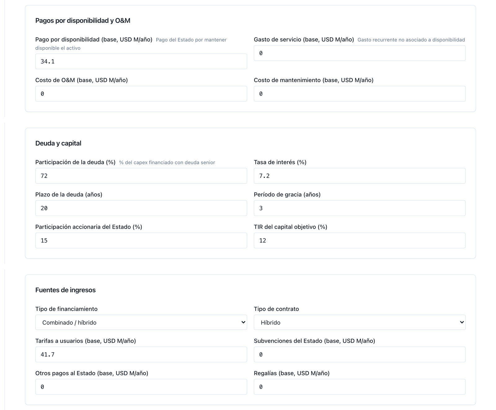
How it is calculated. Each commitment is projected with its own rule —the availability payment with its index from its first year; the equity contribution in the construction years in proportion to that year's investment (in the example, 15 % × 231.7 / 206.7 / 206.7 = 34.8 / 31.0 / 31.0; §4.2)— and is read from the model's series, not recalculated outside it. The equity contribution belongs here, not in step 3: the disbursement is certain in existence; the risk of losing that capital if the company incurs losses is a risk and goes to the matrix of step 3.1. PFRAM 2.0 treats it as a debt guarantee (§2.1); the manual states the difference, and the reconciliation is direct: one reading looks at the flow, the other at the exposure. Supervision is a firm commitment of the State —the contract obliges it to supervise the project for its whole life, and the expense occurs whether or not there is a default— and is projected with the same rule as M1 (step 7): 2 % of total nominal investment per year of operation ◆, from construction completion to the end of the contract, unless the country has its own rate or a priced fiscal-inspection contract (on the Coastal Highway, 2 % × 645.0 = 12.9 per year in 2028-2052: 322.5 in lifetime sum and 118.1 at present value, figures the firm-commitments row of §4 already incorporates). It is recorded in its own row, separate from the availability payment, because the private partner does not receive it and it does not enter the financial liability of step 7; the tool models it with its own field, at its default value unless the contract states its own, with the provenance flag (§5.2).

Decision rule. Performance conditionality does not make a payment contingent. An availability payment with deductions is still a firm commitment: its existence is certain, its amount varies; and in a well-designed contract the probability of paying it is "near certain" (Reference Guide, §2.4.3). What makes an obligation contingent is that its existence depends on an event (GFSM 2014, ¶7.251 and note 71). A construction subsidy conditioned on construction milestones is firm; compensation for a traffic downturn is contingent.

Where teams go wrong. Moving the availability payment into the contingency record "because it depends on performance," which makes the portfolio's largest commitment disappear from the medium-term budget. And the opposite: counting the equity contribution as contingent with probability 1 —two identical series for the same thing— or adding it to the portfolio's maximum exposure (§6.3).

Step 3 — Identify the contingent liabilities

In. The contract clauses that create conditional obligations —guarantees, compensation, rebalancing, termination— and the applicable law (the concessions law, the PPP law, the fiscal responsibility law).

Out. The contract's contingency record: one row per obligation, each in one of two lists.

(a) Valuable —they have an observable state variable and a payment formula in the contract—:

(b) Not valued here —they go to the matrix of step 3.1 with qualitative probability and impact and with the reason they are not valued—: change of law; force majeure without a payment clause; restoration of economic balance; renegotiation; implicit guarantees (the expected bailout with no clause). No figure is assigned to them because they have no state variable or payment formula in the contract; giving them a "reasonable" probability and amount would produce a number with no source that would be added to the ones that do have one.

How it is calculated. By reading clause by clause. An MRG clause has four pieces that a record noting simply "MRG: yes" loses —the floor, its indexation, its window and its price— and sometimes a fifth, the waiver (box 4.11). A termination clause has a basis by cause, and the most frequent cause in the record (concessionaire default) usually has the lowest basis (outstanding debt).

Decision rule. One obligation, one row. The debt guarantee and the termination compensation for concessionaire default cover the same outstanding debt and are mutually exclusive: if the concessionaire defaults, the State pays the debt as compensation or covers the guaranteed fraction as guarantor, not both. Both rows are recorded, but the contract contributes to the portfolio, year by year, the larger of the two —in the maximum and in the expected value—, not the sum. The equity contribution is not contingent (step 2). Every valuable row carries the clause citation; every non-valued row, the reason.

Where teams go wrong. Adding the guaranteed debt and the termination compensation together as the contract's "exposure": in the example, 683.4 instead of 425.4 (§4.4.4). Noting "MRG" without its window or its indexation and valuing a thirty-year guarantee where the contract gives sixteen. And omitting the implicit-guarantee row because "it doesn't exist": the expectation does exist, and the matrix is the place to say it is not valued.

3.1 The fiscal risk matrix

In. The eleven categories of PFRAM 2.0 —governance, construction, demand, operation and performance, financial, force majeure, adverse government action, change of law, financial rebalancing, renegotiation and termination— with their questions (§2.1), and the non-valued rows from step 3.

Out. By category: likelihood (low / medium / high), impact (low / medium / high, with the thresholds in % of GDP the country sets), rating (the product: irrelevant, low, medium, high, critical), mitigation (yes / no) and action priority.

How it is calculated. It is a documented judgment, not a formula: every rating carries one line of support. The rating is read from PFRAM's likelihood × impact grid (figure 7); the priority, from the rating crossed with the existence of mitigation (figure 8).

Decision rule. The matrix does not produce figures that are added to the record. It is where the risks the method does not value in money live, and the evidence that they were thought through; and it is the fifth figure of §1.4: what was not valued and why. A contract with all eleven categories "not assessed" is not on the record, however complete its guarantees are.

Where teams go wrong. Filling in the matrix with "medium / medium" for every row, in one meeting, with no support: it conveys nothing. And its opposite, valuing renegotiation in money "at 30 % probability and 10 % of the investment," adding it to the contingent figure and losing the line between what the contract obliges and what the analyst fears.

Step 4 — Value the firm commitments

In. The nominal calendar from step 2 and the policy discount rate.

Out. Two figures per commitment and per contract, and both are published: the nominal annual profile (the budget and medium-term framework figure) and the present value at the declared rate (the record and stock-ceiling figure).

VP(firme) = Σ_t  firme_t / (1 + r)^t        t = 0 in the base year

How it is calculated. The rate r is a policy parameter —the social discount rate or the public debt rate, depending on the country's framework—, is declared with its provenance and is the same for the whole portfolio. In the example, the workspace's rate, 8 % ◆, with 5.5 % as a sensitivity. The project's cost of capital (WACC) serves the model of step 1 —to know whether the contract closes— not to value what the State owes: discounting the State's obligation at the private rate shrinks it by exactly the premium the private party charges. The 2022 compendium (note 35) discusses whether the local risk-free rate is adequate for payments that occur in a crisis; the manual discounts at the policy rate and says so. When the two-rate rule from the Value for Money analysis is in production, the manual will align with it.

Decision rule. The two figures are always published, with their label: "lifetime sum" is not "present value," and neither one is "the commitment." The rate moves the stock more than any guarantee assumption moves the expected value (in the example, +32 % moving from 8 % to 5.5 %; §4.3): a record that does not state its rate is not comparable with the previous year's or with another country's.

Where teams go wrong. Discounting availability payments at the project's WACC "because it's the model's rate." Comparing the nominal lifetime sum (1,546 in the example) against a stock ceiling defined at present value (490). And changing the rate between two annual versions without recalculating the previous one, so that "exposure went up" when only the rate went down (step 10).

Step 5 — Value the contingent liabilities: maximum, expected value, distribution

In. Every valuable row from step 3 with its state variable read from the model of step 1 (the private partner's revenue series, outstanding debt by year, the projected exchange rate, the compensation basis by year), its contractual parameters (floor, coverage, cause, threshold, notional) and its declared assumptions (revenue volatility, annual default probability, recovery, cumulative termination probability, exchange-rate volatility).

Out. By obligation and by year, three figures:

• the maximum exposure: what the State would pay in the worst case the contract admits —the MRG floor, the guaranteed fraction of outstanding debt, the compensation in full for termination, the notional at the 95th percentile of the exchange rate—; it is a contractual figure, it does not depend on the simulation;
• the expected loss: the average payment over the distribution of the state variable;
• the distribution: 5th / 50th / 95th percentiles, value at risk (VaR) and expected shortfall (CVaR) at 95 %, the probability that the guarantee pays out at least once over its life, and the maximum loss by path;

with seed, number of runs and confidence interval published: seed 42 ◆ and 2,000 paths ◆, the same N throughout the method —in the portfolio record, in the design workshop and in the portfolio band— because two different N's for the same clause produce two different tails by pure sampling, and the ministry would not know which one to sign off on. And every published probability carries its label: annual or cumulative (over the life of the contract). Both conventions coexist in the method —the debt guarantee's is annual, the termination's is cumulative— and are converted into one another with h = 1 − (1 − P)^(1/n) and P = 1 − (1 − h)^n, where n is the number of years at risk; step 5 develops this for each guarantee.

The rule that ties all the methods together. The guarantee is valued on the distribution of its state variable, never on its mean path. On the mean path a well-set MRG is worth exactly zero, and a debt guarantee valued as exposure × probability counts one default every year of a contract that can only default once; the distribution corrects the first one upward and the second one downward (box 4.4.1: 0 → 254.8 and 49.5 → 26.4). A single law does not mean figures go up; it means every clause is valued as what it is.

How it is calculated, by type.

Minimum revenue guarantee. The method's default revenue process is geometric Brownian motion (GBM) ◆, centred on the path of the contract's own model —in every year, the mean of the paths is the base revenue— with volatility σ declared per contract:

R_t^(k) = R̄_t · exp( −σ²·t/2 + σ·W_t^(k) )          k = 1 … N paths, t years from the start
pago_t^(k) = cobertura · máx( 0 , piso_t − R_t^(k) )
esperado_t = (1/N) · Σ_k pago_t^(k)        máximo_t = cobertura · piso_t

If the contract has surplus-sharing above a cap, it is subtracted on the same path: − máx(0, R_t − techo_t) · fracción. Volatility is an assumption declared per contract, with no silent default: if it is not declared, the tool uses a 15 % ◆ reference value and prints it as an undeclared assumption, with the sensitivity table 5 / 10 / 15 / 20 / 30 % next to the figure (in the example, 27.0 / 131.2 / 254.8 / 379.6 / 614.3; §4.4.1). Mean reversion is the declared alternative: it gives a stationary cost instead of one growing with σ√t, and is appropriate when traffic has a long-run level it returns to after a shock (a saturated urban road) rather than an uncertain trend (a new inter-city road). The record uses it only if the contract profile declares it, with its reversion speed and its long-run level next to the volatility; the design workshop offers it and values it, and the record's row states process: mean reversion so the reviewer knows not to compare it with the other rows under the same law. Absent a declaration, the process is geometric Brownian motion.

Convention for the mixed contract. The MRG is compared against the private partner's total revenue —toll plus availability payment (PFRAM's "operator revenue")—, not against the toll alone: the clause guarantees a revenue, and a partner receiving an availability payment has that revenue. The floor is set on whatever the clause says (in the example, 80 % of first-year toll revenue = 44 % of total revenue), and the guarantee is valued against the total. The difference is not a fine one: the same clause on a pure-toll contract costs three times as much as a fraction of the floor (§4.4.1). The record states the convention in the contract profile.

Debt guarantee. Two triggers. By default ◆: on every path the first default is drawn with annual probability PD (1.5 % ◆; D15) and, when it occurs, the State pays the coverage on that year's outstanding debt net of recovery, and the path does not default again:

máximo_t   = cobertura · deuda_pendiente_t                              (cobertura 50 % ◆)
pérdida^(k) = cobertura · (1 − recuperación) · deuda_pendiente_τ(k)     τ(k) = year of the first default
esperado_t = (1/N) · Σ_k pérdida^(k) · 1[τ(k) = t]                       (recuperación 40 % ◆)
P(alguna llamada) = 1 − (1 − PD)^n

By debt service coverage: default occurs on the path when the simulated revenue flow pushes coverage below a threshold; useful when debt risk is the same revenue risk that triggers the MRG, in which case the two guarantees are valued on the same paths. It always uses the contract's actual debt schedule (tranche, grace period, amortization), never a flat debt profile. The debt guarantee's probability is declared annually —that is how rating agencies and default studies measure it, and the one the first-default draw consumes— and is published alongside its lifetime cumulative figure, P(alguna llamada) = 1 − (1 − PD)^n, which is the one step 7 compares against 0.5: at 5 %, a 28-year contract defaults at least once with probability 76 %; at 1.5 %, 34 %; observed rates in project finance run at roughly a third of 5 % (§2.6, Moody's). That assumption alone decides the accounting entry of step 7.

Termination compensation. The probability is declared cumulative over the contract (10 % ◆) and converted into a constant annual hazard rate, so that the sum of annual probabilities is exactly the declared figure:

h = 1 − (1 − P_acum)^(1/n)            p_y = h · (1 − h)^(y−1)          Σ_y p_y = P_acum
máximo_y   = base_y                    esperado_y = p_y · base_y  (along the path) ≈ Monte Carlo

A record that applies the 10 % to every year multiplies the expected value by twenty-five. The basis for compensation is by cause, and the model of step 1 reads it year by year: concessionaire default → outstanding debt (or book value settled as debt); State default → outstanding debt + equity at book value + a fraction of the unearned return (50 % ◆ of the present value of future cash flows to equity); force majeure → debt + equity, no return; or a fixed amount if the contract sets one. This is the row where the distribution does not change the expected value —the event is discrete and the annual probability is the same under both laws (23.9 versus 24.5 in the example)— but it does show what is lost when it happens: VaR 95 of 268.3 and CVaR of 333.9 on an expected value of 24.5 (§4.4.3). Two neighbouring guarantees thus carry two probability conventions —annual for debt, cumulative for termination— and the method keeps them unreconciled, because each is the form in which its source states it: termination's is the one PFRAM and the contracts write down ("10 % probability of early termination"), and converting it to annual for publication would force the reader to undo the conversion. What the method requires is the label next to each figure and the conversion printed whenever the two are placed side by side (h = 1 − (1 − 0.10)^(1/28) = 0.376 %; 1 − (1 − 0.015)^28 = 34 %).

Exchange-rate guarantee. The expected value is the value of an option on the exchange rate (Garman–Kohlhagen, risk-neutral) with the base rate, the threshold, the domestic and foreign rates, the volatility and the notional covered; the maximum is the payout at the 95th ◆ percentile of the exchange rate's lognormal distribution in each year. It enters only if the contract has one (the example does not).

Disputes and arbitrations. esperado = cuantía realista × probabilidad de pérdida, máximo = cuantía reclamada; a provision if the probability exceeds 0.5 ◆ (IPSAS 19), with 0.75 ◆ as "high probable." These are carried at the portfolio level, not the contract level.

Generic guarantees. esperado = máximo × probabilidad, spread over its window of years.

The contract's contingent figure. With the mutually-exclusive rule of step 3, year by year:

máximo_t   = MRG_máx_t + máx( deuda_máx_t , término_máx_t ) + FX_máx_t + genéricas_máx_t
esperado_t = MRG_esp_t + máx( deuda_esp_t , término_esp_t ) + FX_esp_t + genéricas_esp_t

and máximo_t ≥ esperado_t in every year, because they are read from the same series. In the example: peak maximum 425.4 (not 683.4), expected lifetime sum 96.2 (not 119.0; §4.4.4).

Decision rule. Three figures per guarantee, never one; seed, N and confidence interval published; volatility and probabilities named, sourced and labelled (annual / cumulative), with their sensitivity table alongside. And the methodological note that §5 verifies: the same engine, with the same seed and the same N, must value the guarantee both in the portfolio record and in the design tool. If the record values on the mean path and the workshop by simulation, the ministry reads two numbers for the same clause, and no one knows which to sign off on.

Where teams go wrong. Valuing the MRG on the base projection and writing "no expected cost" (§6.1). Valuing the debt guarantee as exposure × probability every year (§6.1). Using the cumulative termination probability as if it were annual. Taking the volatility "from the template" and not printing the table (§6.2). And adding up per-contract VaR as if it were the portfolio's VaR, which is the error of the next step.

Step 6 — Consolidate the portfolio

In. Each contract's annual series from step 4 and step 5 —firm; maximum contingent; expected contingent—, aligned to the horizon of step 0; and the declared correlation structure.

Out. The portfolio's series by year —firm, maximum, expected—, its summaries under two declared conventions, and the portfolio's confidence band.

How it is calculated. The series are added year by year. The summaries:

• Annual peak = the maximum of the portfolio series: the headline figure, the one measured against the ceiling and entered in the memorandum item.
• Lifetime sum = the undiscounted sum of the series: a transparency figure, which is not "total loss" nor "debt."
• Present value of the expected value at the policy rate: the provision figure.

Both summaries are read from the same annual series: maximum ≥ expected under either one, and the sum of per-contract peaks is not the portfolio's peak (in the example, 28,737 versus 27,503, a 4 % difference; in portfolios with dispersed schedules, much more; §4.5). Maximums are not discounted: they are contractual stocks.

The correlated band (base method). A portfolio's guarantees are not called independently of one another: a recession lowers traffic on every road at once, and a devaluation triggers every exchange-rate guarantee. The portfolio is simulated with correlated shocks —block correlation, 0.24 ◆ between contracts in the same sector and 0.12 ◆ between sectors, the two endpoints of the Basel II asset correlation formula (¶272), adopted as a declared convention, not as an estimate—, and the median, the confidence percentile (95 % ◆) and the mean are read by year; at the peak and in the lifetime sum, the VaR and the CVaR. The independent sum (ρ = 0) is presented as a lower bound, and the comonotonic case (everything moves together) as an upper bound. Declarable alternatives: a single ρ, a per-contract matrix, or a common factor tied to GDP. The band's mean should reconcile with the series' deterministic expected value (796 versus 748.9 in the example, within sampling error; previously 639 versus 611.6, with the MRG workbook prior to the correction of the MRG floor's basis, §4.4.1); if it does not reconcile, one of the two calculations is wrong.

Decision rule. The figure that goes into the fiscal risk statement as "contingent loss at 95 % confidence" is the correlated P95 (1,706.7 in the example's peak year), not the sum of each contract's VaR (3,575.2, more than double: it adds tails that do not coincide in time) nor the independent sum (1,471.5). Seed, N and correlation method published with the band; and if the tool reduced N to respond in time, the band says so ("degraded").

Where teams go wrong. Adding up VaR by contract (§6.5). Presenting the maximum as "the sum of peaks" and the expected value as "the lifetime sum" in the same table, which can make the maximum come out smaller than the expected value (§6.4). And taking the band's mean for "the loss" when the tail is the only thing correlation moves.

Step 7 — Classify and report: accounting, statistics, budget

In. The consolidated series from step 6, the per-contract series and, per contract, the control test (who controls what service is delivered, to whom, at what price, and who keeps the asset at termination).

Out. Three outputs from the same record, on the same date, which must reconcile with one another, and the table that reconciles them.

Accounting (IPSAS). By contract, the IPSAS 32 control test (¶9): if the State controls the service and the residual interest, the asset enters its balance sheet with an offsetting liability for the same amount, whether the State pays or the user pays. The liability has two models, and a mixed contract combines them in proportion to what each source pays of the asset: the part the State pays with the availability payment is a financial liability (¶18–19), and each payment is split into finance charge, service expense and amortization (¶21–23), at the rate that settles the liability over the contract term; the part users pay is a liability under the "grant of a right to the operator" model (¶24–26), deferred revenue recognized as the concessionaire collects. An MRG on its own is enough for the contract to carry a financial liability for the guaranteed amount (¶19(b); N10). For contingencies, IPSAS 19: a provision if there is a present obligation, the outflow is probable —"more likely than not": p > 0.5 ◆— and the amount is estimable (¶22), measured at the best estimate (¶44), that is, the expected value at present value; a disclosed contingent liability in a note if possible but not probable (¶35–36), with its gross exposure and its estimated financial effect (¶100); nothing if remote. The note is presented by currency.

The probability compared against 0.5 is the probability that the guarantee pays out at some point over the life of the contract —a rule of this manual— and the annual probability is published in a note, alongside it. The reason is consistency between the test's two halves: the provision is measured at the best estimate of the outflow that will settle the obligation (¶44), which for a guarantee is the lifetime expected value at present value; the probability that decides whether that figure is a provision or a disclosure must be over the same horizon, or the entry ends up comparing one year's probability with twenty-eight years' cost. The probability for the reporting year answers a different question —whether the guarantee will pay out this fiscal year— and goes in the note as such; the medium-term framework's horizon has no accounting definition and is not used. Under this rule, in the example, the debt guarantee is a disclosure at 1.5 % annual (35 % lifetime) and would have been a provision at the previous 5 % (76 %); none of the portfolio's 60 debt guarantees is a provision at 1.5 % (59 were at 5 %), and the 21 MRGs of the pure-toll contracts (63 % and 77 % lifetime in the two boxes of §4) are provisions while the Coastal Highway's (39 %) and the rest of the mixed contracts' are not (§4.6). This rule is also what makes the D15 default defensible: since the classification of almost the whole portfolio depends on the lifetime cumulative figure, a default annual probability cannot be a comfortable marker (5 %) but must be a sourced calibration (1.5 %, in line with observed rates in project finance, §2.6); and a record that replaces it with its own writes down where it got it.

Statistics (GFSM 2014 / ESA 2010). By contract, economic ownership by risks and rewards (GFSM, appendix 4, box A4.4) or the risks-and-rewards test under the European System of Accounts 2010 (ESA 2010) with its rules for return to the balance sheet —guarantees, public financing, termination clauses (MGDD 6.4)—; in practice, "broadly consistent" with IPSAS 32 (¶A4.63), and the example arrives at the same place by all three routes (§4.6). From the record come the government's statement of operations and balance sheet: investment expenditure and net lending in the construction years, financial liability, non-financial assets, net worth; the equity contribution as a financial transaction; and the explicit contingent liabilities as a memorandum item at nominal value (6M61 guaranteed debt, 6M63 other explicit contingent liabilities; ¶4.47, ¶7.255), with the valuation-method metadata note 74 requires.

Budget. The firm commitments by year, in the medium-term framework and in the annual budget law; the contingent expected loss as a provision, a contribution to a contingency fund (Colombia) or a guarantee spending ceiling (Chile: annual appropriation); the maximums as an informational item. Firm and contingent figures are never added together in a single line.

How the reconciliation is calculated. A table per contract and per portfolio with each figure and where it is written. For the example there are ten figures for one obligation (§4.6): the nominal sum of the availability payment (budget), its present value (record and ceiling), the equity contribution (financial transaction), supervision in nominal sum (budget, current expenditure) and the full firm commitments at present value (record), the peak IPSAS 32 financial liability (balance sheet), total GFS liabilities (augmented debt), the maximum contingent figure (memorandum and ceiling), the expected contingent figure in lifetime sum (provision or spending ceiling) and at present value (IPSAS 19 note). None of these is "the" figure; the reconciliation explains why the IPSAS liability is not the budgetary commitment, nor GFS debt, nor the contingent exposure. Every present value in the method —the firm commitments of step 4, each guarantee's expected value, the note's provision— is discounted under a single convention: from the base year, t = 0 undiscounted, as in step 4; no expected value is discounted twice. It is a convention, not a truth —discounting from the end of the first year is equally valid— but a figure discounted two different ways in two parts of the same report reconciles with nothing: without this discipline, the contract's three guarantees would have been worth 40.4 row by row from the base year (28.6 under the mutually-exclusive rule) against 37.4 under the convention guarantee tools used to carry (§4.4.4), and under the previous 5 % the debt guarantee would have been a provision with the note discounting it once more (37.1 from the base year, 34.3 in the workshop, 31.8 in the note). The platform now unifies its modules under this convention (§5.5).

Decision rule. The three outputs are produced from the same record on the same date, and the reconciliation is part of the report, not an annex. A ministry that publishes the IPSAS liability in March, the budget in October and GFS debt in June, each from a different file, has three figures and no reconciliation (§6.6). The control test is documented by contract, with its result and its reason; the ESA classifier is also run as a second opinion, and any divergence is noted.

Where teams go wrong. Leaving an availability contract off the balance sheet "because construction risk sits with the private party" —the IPSAS 32 test is about control, not risk—. Recording the debt guarantee as a provision at maximum exposure instead of the expected value. And counting the nominal sum of availability payments as public debt: the debt is the financial liability, not the flow.

7.1 The fiscal risk statement

In. The portfolio series from step 6 —the firm + contingent pair— and the guarantee record from step 5 with its assumptions.

Out. The PPP chapter of the annual fiscal risk report, with the structure the Chilean contingent-liabilities report has used since 2007 and that the Fiscal Transparency Code (2019, principles 3.2.3 and 3.2.4) requires: for each mechanism —MRG, debt guarantee, termination, exchange rate, disputes—, the nature of the obligation and its beneficiaries; the maximum exposure; the expected value with the method that produced it (simulation, seed, N, declared volatility); the present value of both; the year's payments and fees collected; and the difference against the previous report, by cause (step 10).

Decision rule. The portfolio enters the statement as the firm + contingent pair, once, without double counting against the budget chapter (which already carries the firm figures) or the stress-test chapter (which carries shocks on the same portfolio): if the same contract appears in two chapters, one of the two nets it out and states by how much. Assumptions travel with the figure: "MRG: expected value 254.8" without "volatility 15 %, declared, seed 42, N 2,000" is not a publishable figure.

Where teams go wrong. Publishing the maximum as "the risk" without the expected value, or the expected value without the maximum; and publishing the chapter without the list of what was not valued (the matrix of step 3.1), which is the part an informed reader looks for first.

Step 8 — Ceilings and affordability

In. Nominal GDP (or fiscal revenue) projected on the same price base as the indexed payments; the commitments ceiling (% of GDP or of revenue; 5 % ◆ in the example); the contingencies ceiling (% of GDP; 3 % ◆); the alert threshold (80 % ◆ of the ceiling); and the scoring rule.

Out. By year: exposure scored against each ceiling, in % of GDP and in % of the ceiling; the years of breach and of alert; and the alerts from the workspace's own rule (maximum stock in money, % of GDP).

How it is calculated.

( firmes_t + esperado_t ) / PIB_t   against ceiling 1        máximo_t / PIB_t   against ceiling 2

This is a flow ceiling (every year against that year's GDP); a stock ceiling —such as Peru's 12 % of GDP, on the present value of firm commitments and quantifiable contingent liabilities— is scored with the portfolio's present value against the base year's GDP. Against the commitments ceiling go the full firm commitments plus the full expected contingent figure: availability payment, service payments, subsidies, equity contribution and supervision (step 2), plus the expected loss of the MRG, the debt guarantee, termination, the exchange-rate guarantee and generic guarantees (step 5, under the mutually-exclusive rule). This reads the ceiling as the year's expected expenditure: what the budget should set aside if every guarantee behaved like its mean. Leaving out the equity contribution because "it's a financial transaction," or the expected debt and termination figures because "they're remote," turns the ceiling into a ceiling on whatever is convenient; in the example, the portfolio moves from 0.75 % —what the dashboard scored before aligning with this rule— to 0.97 % of GDP in its worst year once everything is counted (§4.7): 0.18 pp is the portfolio's supervision cost and 0.03 pp is the expected debt and termination figures (the equity contribution had already ended in 2032). Against the contingencies ceiling goes the contractual maximum, which is what the ceiling limits: how much can be promised.

Decision rule. It is stated what goes against the ceiling —firm + full expected value against the commitments ceiling, maximum against the contingencies ceiling, and whether the peak year's correlated CVaR is also published— because the verdict depends on the rule, not on the portfolio: for the example, the maximum breaches the contingencies ceiling in twelve years (6.15 % of GDP in 2030), the peak year's correlated CVaR 95 stays below a third of the ceiling, and firm plus expected is at 16 % of the commitments ceiling (§4.7). A ceiling on the maximum is met by cutting guarantees, not by reducing risk; a ceiling on the expected value is met by lowering the declared volatility, which is worse (Austral, The Pipeline Under the Ceiling, §2-3 and §8). And the flow ceiling is not enough without the full firm envelope —the half almost nobody publishes— (Austral, The PPP Budget Nobody Publishes). It refers back to step 12 of M1: a contract passes only if it passes its Value for Money test and fits under the ceiling in every year.

Where teams go wrong. Scoring the series' average against the ceiling, which makes the peak year disappear. Scoring a nominal 2050 series against today's GDP. And "meeting" the ceiling by switching the rule —from the maximum to the expected value— between two reports without saying so.

Step 9 — Sensitivity and stress

In. The base case from steps 4 through 8; the shocks —construction cost, operating and maintenance costs, revenue, interest rate, inflation, exchange rate, and a compound macro shock—, in points or in percentage, by contract or by portfolio; and the valuation parameters of step 5 (volatility, default probability, termination probability, coverage).

Out. By contract, a tornado: each variable moved on both sides and the chosen metric recalculated —the State's NPV, maximum financial liability, maximum contingent figure, maximum debt, coverage—, with bars sorted by width. By portfolio, the base / shock / delta table for each series under a shock, and the band from step 6 recalculated under the macro shock.

How it is calculated. Every bar is a complete recalculation of the contract —model, firm commitments, guarantees— with a single variable moved, and with the same random paths (common random numbers) across all runs, so that the difference is the shock's and not chance's. Two properties of the response the analyst must know how to read: the stocks (maximum financial liability, maximum contingent figure) are contractual figures and are not discounted, so a discount-rate shock does not move them and is not reported; and on the maximum contingent figure only the variables that change outstanding debt or the floor move it (construction cost), while on the State's NPV inflation and revenue dominate (§4.8). Two definitions the method fixes. The "revenue" shock acts on user revenue —toll, tariff, demand—, not on the availability payment, as in M1: the availability payment is not an uncertain revenue for the private partner but a commitment of the State, and it has its own shock, the inflation one (and the exchange-rate one, if it is indexed). A "revenue" shock that also scales the availability payment mixes two things together: in a mixed contract, more revenue would make the State's NPV worse, which is not a property of the contract but of a badly defined shock: the tool does it this way today, and §5 states it as a limitation. And higher inflation cheapens the MRG when the toll follows macro inflation and the floor follows a fixed contractual indexation (+2 pp of inflation lowers the portfolio's expected MRG from 9,137 to 4,389). An MRG protects against a traffic downturn, not against inflation.

Decision rule. The tornado is run on the metric the ceiling scores (step 8), not only on the NPV. And the sensitivity to valuation assumptions —the volatility table, the default probability at 1.5 / 5 %, the termination probability— is published alongside the sensitivity to inputs: in this record the assumption moves more than the input.

Where teams go wrong. Reporting a discount-rate shock on the maximum contingent figure (zero, by construction) as "robustness." Running the tornado with a different seed per bar and reading the noise as sensitivity. And omitting the volatility row from the tornado because "it's not a contract input": it's the one that moves the figure the most.

Step 10 — Monitor and update

In. The previous year's record, with its version and date; the year's events —financial closes, guarantee calls and payments made, renegotiations and supplementary agreements, awards, terminations, new contracts—; actual data (traffic, availability payments settled, deductions); and the revised assumptions (volatility, probabilities, rate).

Out. The year's record, with version and date, and the difference against the previous version explained by cause: (1) new contracts and expired contracts; (2) events (a refinancing changes outstanding debt and, with it, two guarantees); (3) change of assumptions (volatility, probabilities); (4) revaluation (policy rate, macro); (5) the passage of time (one less year of life). Plus the threshold alerts of step 8 and the schedule for the next update.

How it is calculated. The complete previous version —inputs and results— is saved before anything is touched; the changes are applied by cause, one at a time, recalculating after each one, and the difference from each recalculation is attributed to that cause. The order matters little for the total and a great deal for the attribution: it is stated. In the example, four versions separate out +93.7 from volatility, +1.0 from a refinancing and +185.0 from the rate on the firm commitments (§4.8); without them, "exposure went up" is all the next report could say. A renegotiation that alters the allocation of risks is, under ESA 2010, "the cancellation of one contract and the creation of another" (MGDD ¶74): it is recorded as a write-off and a new entry, not as an adjustment.

Decision rule. Every published figure carries a version and a date, and the previous version is never overwritten. A record with no versions is not auditable: it cannot explain its own difference. The tool's default assumptions (◆) that the record has not replaced with its own are listed in each version as such.

Where teams go wrong. Overwriting last year's file (§6.7). Changing three things at once —rate, volatility, a new contract— and attributing the whole difference to the new contract. And updating only the contracts "that changed": the passage of time and the macro environment change all of them.

3.11 Summary on one page

Reviewer's checklist. Ask for: (1) the perimeter, the reporting currency, the base year and the horizon, in one line; (2) the contingency record with one row per obligation, the clause cited in every valuable row and the reason in every non-valued row; (3) the revenue volatility of every MRG, named and sourced, with its 5/10/15/20/30 % table printed; (4) the annual default probability, the recovery rate and the cumulative termination probability, each with its label (annual / cumulative), its provenance, and which ones are default values ◆; (5) the seed, the number of runs and the confidence interval for every guarantee and for the portfolio band; (6) the convention for every portfolio figure —annual peak or lifetime sum— printed next to it, and that maximum ≥ expected value under both; (7) the IPSAS 32 control test documented by contract, with the finance charge–service expense–amortization split; (8) the IPSAS 19 note by currency with the lifetime probability that decided each entry and the annual figure in a note, all at present value from the base year; (9) the IPSAS–GFS–budget reconciliation table of the same date; (10) the scoring rule for each ceiling (firm + full expected value; maximum); (11) the version, the date and the difference by cause against the previous version. A record that cannot deliver all eleven points is not ready to be published, however good its figures look.

4. Worked example: Coastal Highway, a mixed contract inside a portfolio of 81

This section walks through the eleven steps of §3 on a complete contract and then places it inside its portfolio, with the starting figures, the result of each step and the reading Finance would give each figure. The contract is generic — there is no client data — and is one of the 81 that the guest workspace ships as the demonstration portfolio of the "Republic of Andolar", so that the reader can reproduce every number (annex 4.A) and the screenshots in §5 show exactly this case. Every figure comes from running the platform's engine on that portfolio, along the same path the screens use: one model per contract, guarantees valued by simulation with seed 42, 2,000 paths, a declared revenue volatility of 15 %, an annual default probability on the guaranteed debt of 1.5 % (the tool's default value) and a declared recovery of 40 %, and the workspace's policy rate, 8 %, with 5.5 % as a sensitivity. None is calculated by hand: the grantor's supervision cost, which the method had to add separately until September 2026, is now modelled by the tool as its own field on the Costs tab, at its default value (2 % of investment per year of operation) unless the contract declares its own. Figures in millions of US dollars (US$ M) unless stated otherwise; "peak" is the maximum of an annual series and "lifetime sum" the undiscounted sum of the series, as Step 6 defines it.

4.0 The contract and why it serves as the example

The contract. The dual-carriageway expansion of the 80 km Coastal Highway, procured as a mixed PPP: the concessionaire designs, builds, finances, operates and maintains the road for 28 years (2025–2052, three of construction), charges a toll to users and additionally receives an availability payment from the State while the road meets the service standards. Investment is US$ 645 M (620 of works and 25 of land); the State takes 15 % of the concessionaire's equity (an equity contribution of 96.8 across the three construction years), guarantees 80 % of the toll of the first operating year as a minimum revenue guarantee (MRG), guarantees 50 % of the outstanding debt of the senior tranche, and undertakes to compensate early termination for concessionaire default with the book value of the assets, which the contract settles as outstanding debt. In addition, as in every contract, the State supervises compliance with the standards during operation, and that cost is its own (2 % of investment per year of operation, the M1 rule). There is no exchange-rate guarantee: revenues and debt are in local currency and there are no imported components.

Why a mixed contract. It is the only type that has, at once, firm commitments and the three guarantees the method teaches. A pure availability contract has firm commitments and a debt guarantee but no MRG (the hospital in box 4.10); a pure toll contract has an MRG and termination but neither an availability payment nor, in the demo, a debt guarantee (the corridor in box 4.9). The mixed contract shows all four figures from §1.4 — firm, maximum, expected and band — and the fifth, what is not valued. And it has two further didactic virtues that the example exploits:

1. It shows what an MRG is worth when it is set correctly. The floor sits below base revenue in every year, so the guarantee does not pay in the base case — valued on the mean path it comes to exactly zero — and its entire expected cost, 254.8 in lifetime sum, comes from revenue volatility. That is the point §1.5 anticipates and §6.1 exploits. The demo portfolio's calibration was corrected to make this so; the earlier calibration, in which the floor eventually caught up with a flat toll, is kept as a stress variant and shown in box 4.4.2, because it teaches the opposite.
2. It shows the convention that decides what the floor is compared against. In a mixed contract the MRG floor, set on the toll, is compared with the demand revenue that the guarantee insures — the toll, without the availability payment, which is deterministic and cannot trigger it — by the platform's default (mrg_floor_base = "demand"); declaring "total" instead compares it with the partner's total revenue, PFRAM's reading ("partner revenues"). With the declared base, the 2028 floor of 37.3 is 80 % of the toll and the guarantee costs almost the same, per unit of floor, as the same clause on a pure toll contract (4.4.1); with the total base the availability payment, which can never move, covers the floor every year and the guarantee is worth exactly zero (§4.4.1). A register that does not declare the base is valuing a different guarantee without saying so.

The price of those advantages is also stated: the contract's expected contingent liability is small next to its firm commitment (283.0 against 1,965.4 in lifetime sum), and of the three guarantees only the MRG crosses the provision threshold: it pays at least once in 28 years with 79 % probability under the demand base (4.6); the debt guarantee, valued with the default 1.5 % annual default probability, pays with 35 % probability and goes to the note, like termination. With the 5 % a year the tool carried until September 2026 the debt guarantee would also have been a provision (76 %); annex 4.A keeps both versions. An example with more expensive guarantees would have been more striking and less representative of what a register actually finds.

4.1 Steps 0 and 1: perimeter, contract profile and model

Perimeter (Step 0). Reporting entity: the central government of Andolar. Contracts: the 81 signed contracts of the demo portfolio, all tagged signed. Reporting currency: US dollars (Andolar's peso converts at 850 per dollar on the currency screen; the example presents everything in US$ M). Base year 2025; horizon to the end of the portfolio's longest contract, 2061 — not that of the medium-term framework. Policy rate: 8 %, the workspace's, declared as a policy parameter and not as the project's cost of capital.

Contract profile (Step 1). The model's inputs, as stored by the contract's Government tab and Guarantees tab:

Figure 4.1 — Coastal Highway's profile, Costs, Financing and Revenue tabs: availability payment 34.1, State's equity stake 15 %, user tariffs 41.7 (in production the Government tab shows the contract's GFS statements).

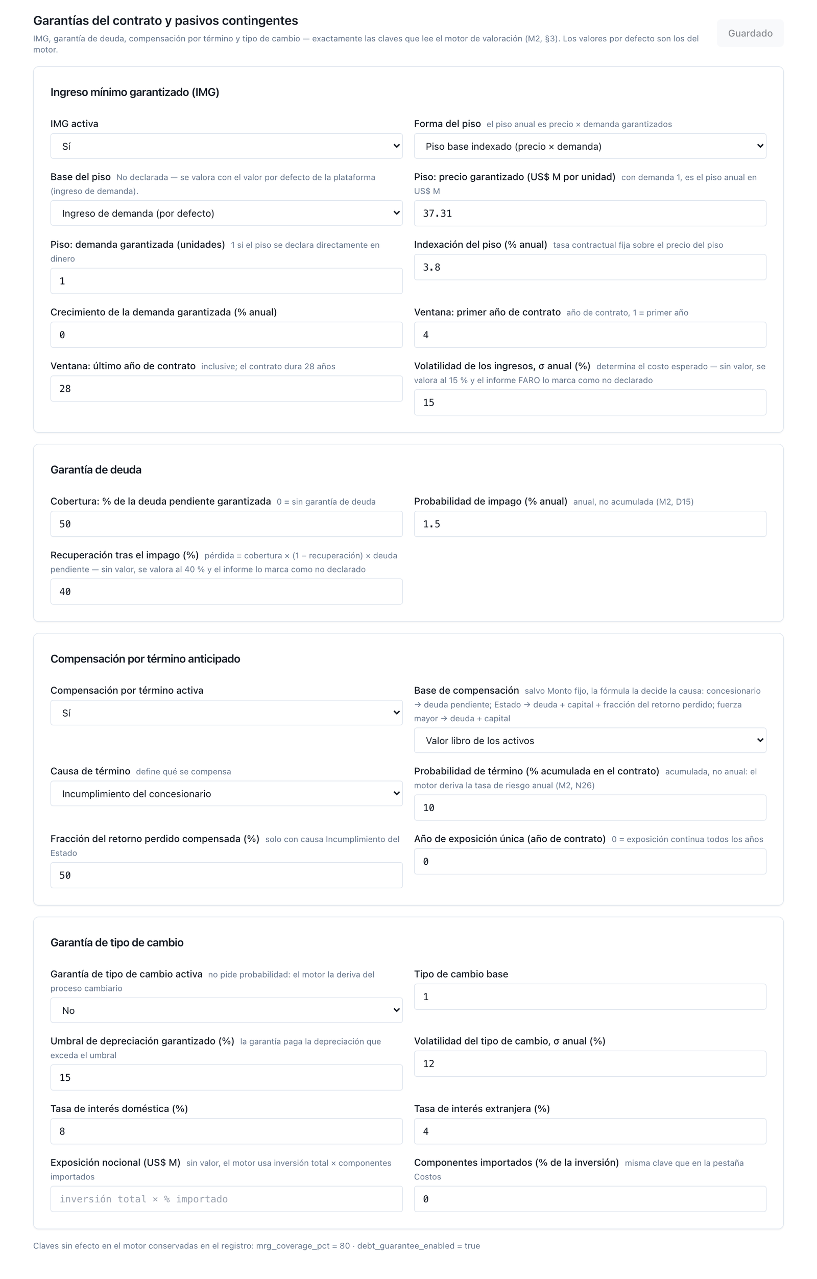
Figure 4.2 — Coastal Highway's Guarantees tab: MRG active (floor 37.31 indexed at 3.8 %, σ 15 %), debt 50 % / 1.5 % annual / 40 % recovery, termination for concessionaire default at book value, 10 % cumulative.

The contract's model. From those inputs the engine builds the annual series from which every obligation is read — it is one model, not a separate guarantees spreadsheet:

Lifetime sums: availability payment 1,546.1; toll 1,890.7; debt service 870.1. The private leg closes: average debt service coverage 2.91 and project IRR of 10.9 %. It is worth checking this before valuing guarantees, for the same reason M1 requires it before comparing: a debt guarantee on a contract that does not finance itself is valuing a contract nobody would sign. Outstanding debt reaches its maximum, 394.7, at the close of construction in 2027 and amortises on an annuity basis through 2051; that profile is the state variable of two of the three guarantees.

4.2 Steps 2 and 3: the firm commitments and the contingency register

The firm commitments (Step 2). Four items, all certain in their existence: the availability payment (38.1 in 2028 growing with inflation to 93.3 in 2052; its performance conditionality — the deductions — does not make it contingent), the equity contribution (96.8 during construction: the State disburses its 15 % of equity with certainty, even though PFRAM 2.0 treats it as a debt guarantee, §2.1; the risk of losing that equity goes to the matrix), the grantor's supervision cost — 12.9 a year from 2028 to 2052, 2 % of total nominal investment per year of operation, the same rule as M1: the tool models it with its own field, on its own row and outside the financial liability, because it is a current expenditure of the State and not a payment to the concessionaire — and the construction subsidy, which is zero in this contract. There are no payments for State-provided services.

The contingencies (Step 3). One obligation, one row; and each row on one of the two lists:

(Coastal Highway's Guarantees tab: figure 4.2.)

The no-duplication rule is already visible here: rows 2 and 3 cover the same debt — if the concessionaire defaults, the State pays outstanding debt as compensation or covers half of it as guarantor, not both — so each year's contract maximum is the greater of the two, not their sum. With the three rows summed the maximum peak would be 683.4; the register's is 425.4 (4.4.4).

The risk matrix (Step 3.1). Rows 6 to 10 are recorded in PFRAM's eleven-category matrix with likelihood and impact on three levels, mitigation and priority. The demo portfolio ships the matrix unassessed (every cell "not assessed"); the example fills it in for this contract as an illustration, and those five ratings are the only assumption in this section that does not come from the engine:

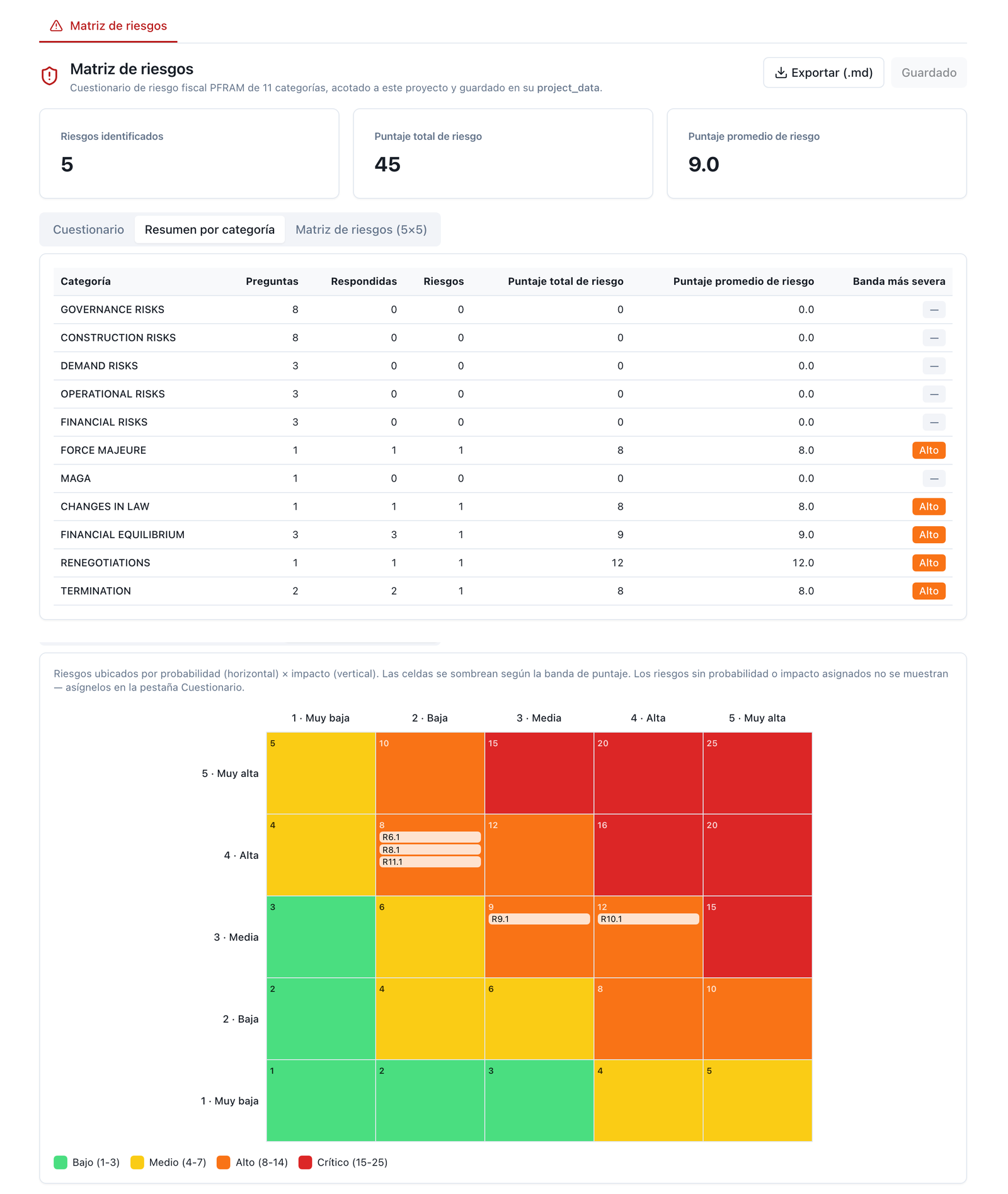
Figure 4.3 — Coastal Highway's risk matrix with the five rows from 4.2: renegotiation 12 (the highest), the rest 8–9; the platform scores on a 5 × 5 grid and groups the five into the High band.

The matrix is where the fifth figure of §1.4 lives: what was not valued, and why. In this contract what is not valued is renegotiation, which the experience of concessioned highways places in the most probable category (§2.5), and which none of the three guarantees covers.

4.3 Step 4: the value of the firm commitments

The nominal profile goes to the budget; the present value at the policy rate goes to the register and to the stock ceiling:

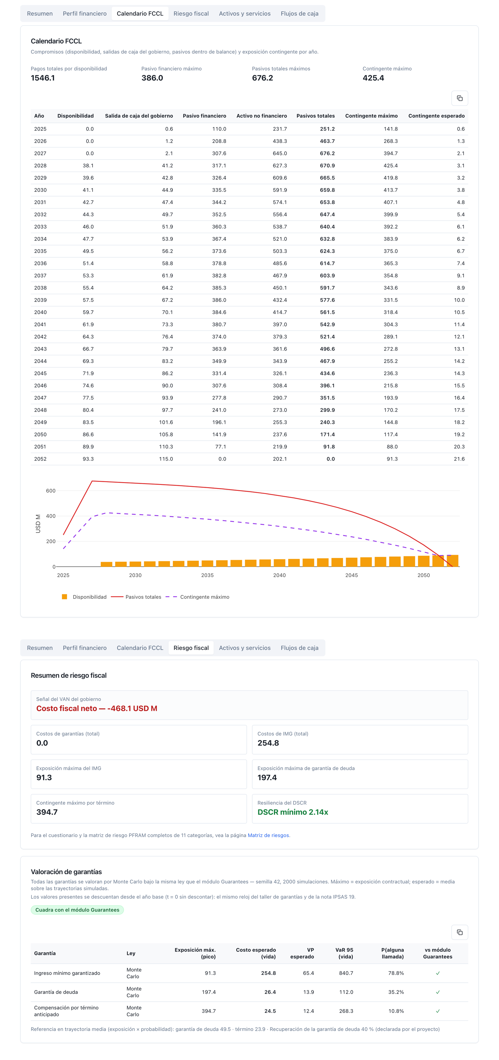
Figure 4.4 — Coastal Highway's FCCL: schedule 38.1 → 93.3, peak financial liability 386.0, total liabilities 676.2, maximum contingent 425.4; guarantee valuations 254.8 / 26.4 / 24.5 (floor base: demand, default) with the ✓ reconciliation mark on all three rows ("Matches the Guarantees module").

Four readings. First: the lifetime sum is nearly three times the PV at 8 % — the PV of the availability payment is 31.7 % of its nominal sum — and the two figures answer different questions: how much the budget will pay (1,965) and how much the obligation is worth today (698). Second: the rate moves the firm stock by 32 % (from 697.8 to 920.2 moving from 8 % to 5.5 %), more than any of the guarantee assumptions moves the expected contingent liability; the register must state which rate it uses and where it comes from. Third: the equity contribution is barely discounted — it is paid in the first three years — and so it weighs more in the PV (12.9 % of the firm total) than in the lifetime sum (4.9 %). Fourth: supervision, which no grantor financial statement records as a liability because it is current expenditure, is 16.9 % of the firm total at PV (118.1) and 16.4 % in lifetime sum (322.5): a register that omits it because "it is not paid to the concessionaire" leaves out a sixth of what is certain. The four figures are the ones the tool publishes.

4.4 Step 5: valuing the contingencies

4.4.1 The MRG

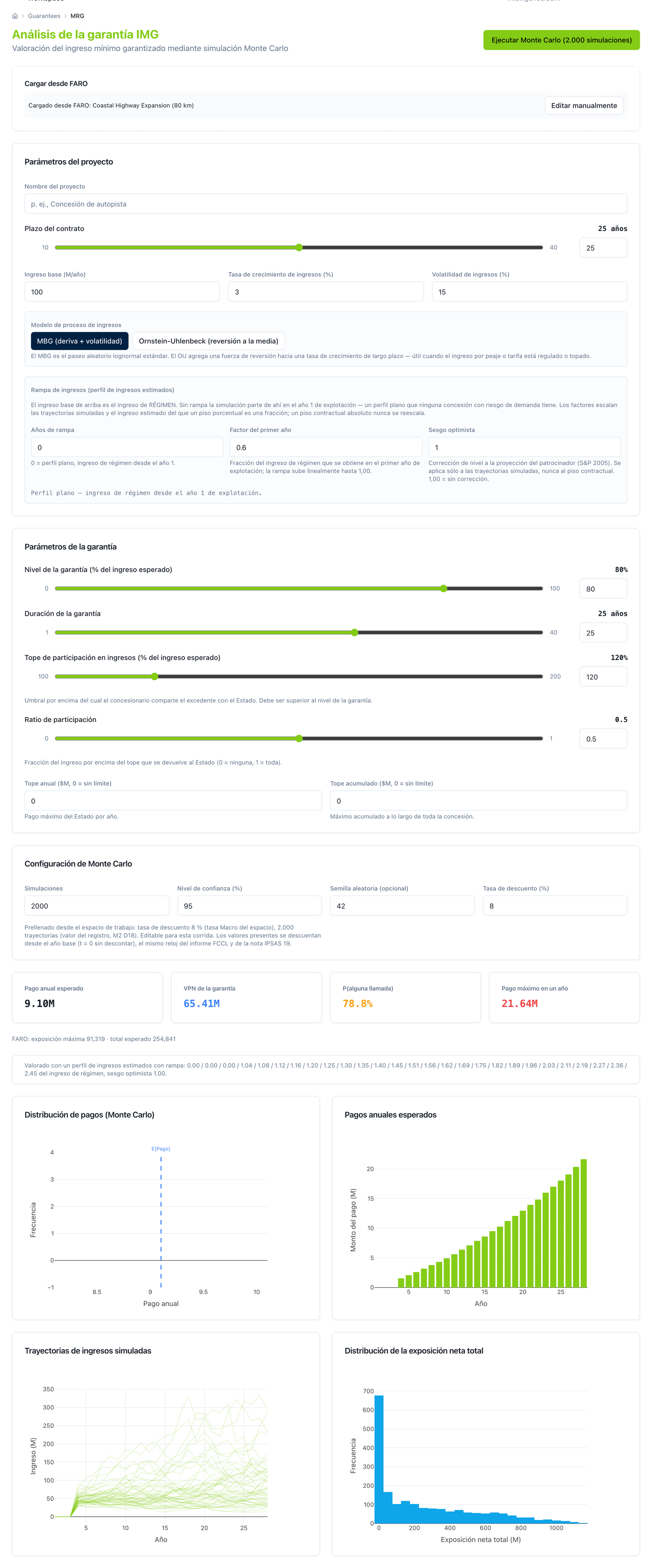
Figure 4.5 — Workshop MRG with "Load from FARO": Coastal Highway's absolute and indexed schedule loaded with one click; guarantee NPV 65.41, P(any call) 78.8 %, maximum payout in a single year 21.64 — reproduces the exact engine figures (254.8 / 65.4 / 78.8 %, §4.4.1).

The state variable is the partner's total revenue, and the simulation models it as a geometric Brownian motion centred on the contract's own model path — in every year, the mean of the 2,000 paths is the total revenue from the 4.1 table — with the declared volatility of 15 %. The guarantee's payout on each path and year is max(0, floor − revenue), and the expected cost is its average:

Floor in lifetime sum 1,512.6; expected cost in lifetime sum 254.8 (16.9 % of the floor); at present value at 8 %, 65.4; probability that the guarantee pays in at least one year, 78.8 %. The cost grows over time even though the floor is the same fraction of base revenue every year, and it is worth understanding why before interpreting it: the Brownian process that simulates the partner's revenue is centred on demand revenue — the toll, the only part that can move — and not on total revenue; with the σ√t dispersion of that smaller process, a floor set at 80 % of the toll turns out to be plausible to cross much sooner than it looked when the same volatility was applied to a total revenue inflated by an availability payment that never moves. This is not a calibration of the contract but a property of the chosen process and base; a mean-reverting process — which the guarantee design tool offers — would give a stationary cost.

The mixed-contract finding. The floor is 80 % of the toll, and the guarantee is valued against the demand revenue that toll represents — the "demand" base, the platform's default — not against the partner's total revenue. That is also what the contracts say: the clause guarantees toll revenue, and the availability payment is a separate, certain obligation that cannot trigger or protect it. The consequence is that the availability payment stops "diluting" the floor: the same clause — 80 % of first-year revenue, same volatility, same life — on a pure toll contract in the portfolio, the 45 km Southern Bypass, costs 15.4 % of its floor in lifetime sum and pays with 77 % probability; on Coastal Highway, mixed, it costs 16.9 % and pays with 78.8 % — practically the same, because in both cases the floor is compared with the same class of volatile revenue. Anyone registering the MRG of a mixed contract by comparing the floor with total revenue — PFRAM's convention, and the one this example used before this correction — is valuing a guarantee protected by a payment that never protects it: that is the reading that made Coastal Highway look cheap, and it was the artefact.

The floor-base rule (17-09-2026). By default, the MRG floor is compared with the demand revenue that the guarantee insures — the toll, without the availability payment — because that is the only thing the clause can protect; declaring mrg_floor_base = "total" in the contract profile instead compares it against the partner's total revenue, adding the availability payment as a fixed figure after simulating, never inside the simulation (the guarantee's volatility is always centred on the toll, whichever base is declared). On Coastal Highway, the demand base — the default, with nothing declared — gives 254.8; the total base gives exactly 0.0, because the availability payment alone (38.1 to 93.3) already exceeds the floor every year. The figure this example published before this correction, 68.0, is not a third legitimate reading: it was what came out of centring the guarantee's volatility on total revenue — the toll and the availability payment together — so that part of the "cushion" protecting the floor came from a payment that can never fall. It remains documented as an artefact, reproducible only as a historical reference, not as one more convention among those the register may choose.

The volatility sensitivity table. Volatility is an assumption declared per contract, and the report prints it next to the table that shows its leverage:

From 10 % to 20 % the cost is multiplied by 2.9. No other assumption in the register has that leverage, and that is why the method requires the 15 % to be a figure written by someone with a name, not a value the engine set because the cell was empty.

Box 4.4.1 — The same MRG valued two ways. Valued on the mean path — the base revenue in the table, with no distribution — Coastal Highway's MRG costs 0.00 across the 25 years: the floor sits below base revenue in every one of them and max(0, floor − base revenue) is always zero. Valued on the distribution, it costs 254.8. The two figures describe the same clause. The first is what any register produces that projects a single traffic path and subtracts the floor — most of them — and is the reason minimum revenue guarantees appear in so many reports as obligations with "no expected cost". The second is the only one that answers the §1.4 question. With the debt guarantee the opposite happens: the mean path gives 49.5 and the distribution 26.4, because the mean path counts a default in each of the 28 years of a contract that can only default once, and does not discount the recovery (4.4.2). And with termination the two rules agree (23.9 against 24.5): the event is discrete and the annual probability is the same under both. A single valuation rule does not mean the figures go up: it means each guarantee is valued on its distribution, and the distribution corrects in whichever direction is appropriate.

Box 4.4.2 — The MRG "that bites": the indexed floor over a flat toll. Before its recalibration, the demo portfolio had flat tolls — 41.7 every year — and the MRG floor indexed at 2 %. On Coastal Highway the floor (33.4 in 2028, 53.7 in 2052) caught up with the toll around 2042; with the floor's demand base, the availability payment does not protect it, and this stress variant costs 268.9 by simulation in lifetime sum (0.00 on the mean path: the floor stays below the modelled toll). The contract where the floor truly bites is the Southern Bypass, a pure toll contract: there the floor of 43.4 indexed at 2 % crosses the flat toll of 54.3 in 2041 and, from that year on, the guarantee pays in the base case — 18.1 in lifetime sum with no volatility at all, 3.5 in 2050 alone — and 268.6 by simulation with a 87 % call probability. That is the signature of a badly set MRG: a positive expected cost on the mean path. A well-set MRG costs only for volatility; a badly set one costs for design as well, and a register that values on the mean path catches the second and is blind to the first. The variant is kept in the tool as a stress case, not as a calibration, and §6.1 returns to it.

4.4.2 The debt guarantee

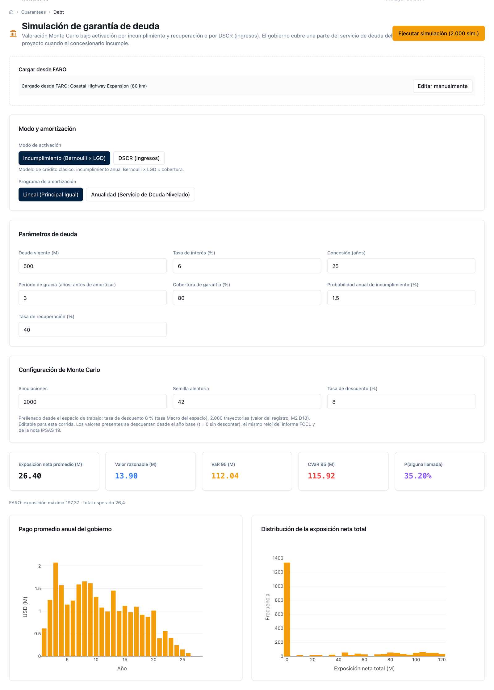
Figure 4.6 — Workshop debt guarantee with "Load from FARO": the actual drawdown schedule (141.8 → 394.7) loaded with one click; average net exposure 26.40, fair value 13.90, VaR 95 112.04, CVaR 95 115.92, P(any call) 35.20 % — reproduces the exact engine figures (26.4 / 13.9 / 112.0 / 35.2 %, §4.4.2).

The state variable is the outstanding debt from the contract's actual schedule, and the event is default. On each path the engine draws the first default with the 1.5 % annual probability — the profile declares it as annual; termination's is cumulative —; when it occurs, the State pays the coverage (50 %) on that year's outstanding debt, net of the recovery (40 %), and the path does not default again. Each year's maximum exposure is the contractual figure — half the outstanding debt — and does not depend on the simulation:

Peak maximum exposure 197.4 (2027); lifetime-sum expectation 26.4 (PV at 8 % from the base year, 13.9); maximum loss per path 118.4 (= 50 % × 60 % × 394.7: the guarantee can never cost more than a default at the close of construction); lifetime VaR 95 112.0. The probability that the guarantee is triggered at least once in 28 years is 1 − 0.985²⁸ = 34.5 % (35.2 % in the simulation), and that is the figure that decides its accounting treatment (4.6). It is worth reading it carefully: the 1.5 % a year is the tool's default value, not a calibration of the contract. It sits in the range of annual default rates observed on project finance loans (§2.6, Moody's), and that is why it replaced the earlier 5 % in September 2026, under which the same guarantee cost 62.5 in lifetime sum and paid at least once with 76 % probability — three out of four contracts so guaranteed defaulting; annex 4.A keeps both versions. A reasonable default value is still a default value: whoever registers this contract must write in their own.

4.4.3 The termination compensation

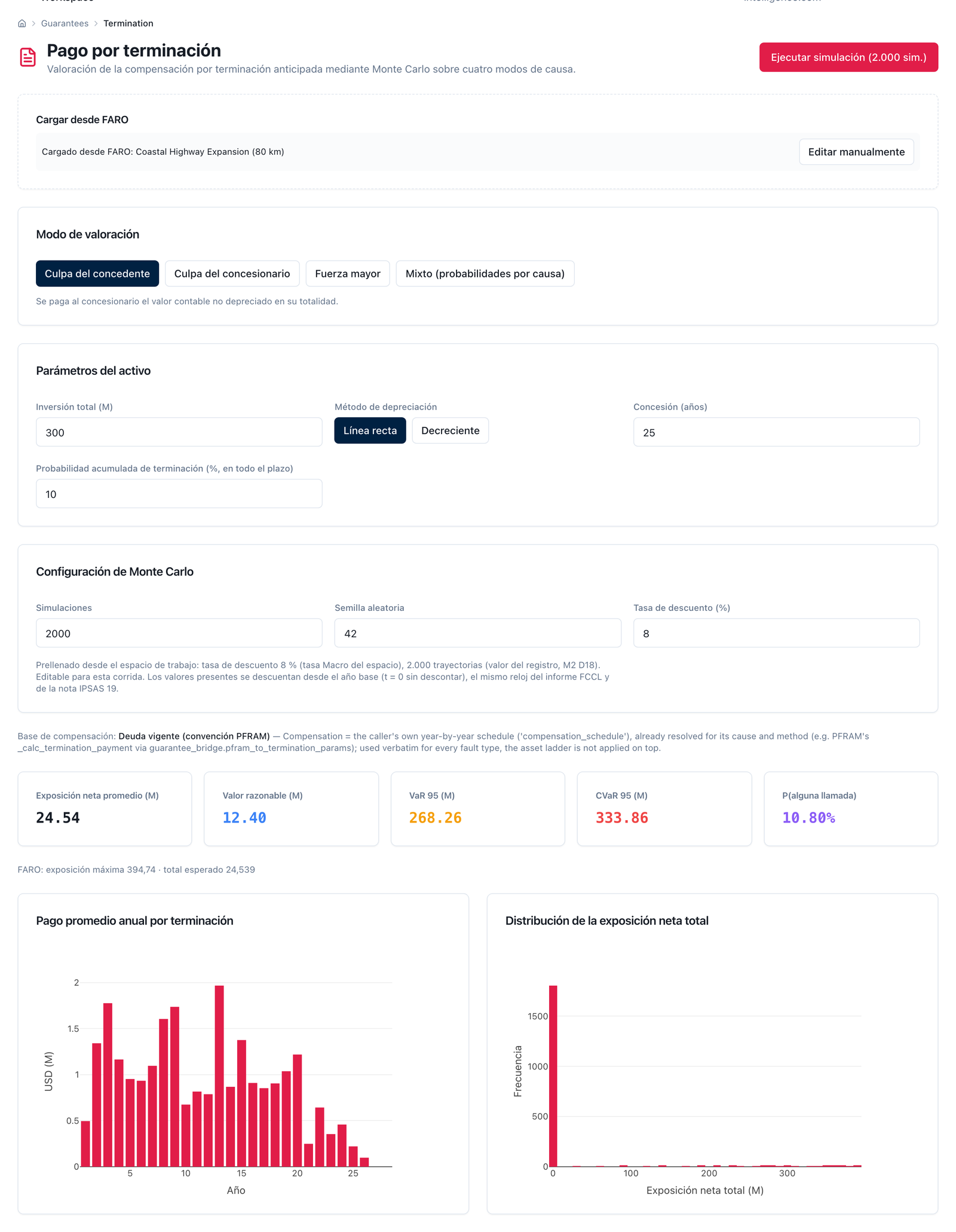
Figure 4.7 — Workshop termination compensation with "Load from FARO": 645 on a straight line, 28 years, printed base "Outstanding debt (PFRAM convention)"; average net exposure 24.54, fair value 12.40, VaR 95 268.26, CVaR 95 333.86, P(any call) 10.80 % — reproduces the exact engine figures (24.5 / 12.4 / 268.3 / 10.8 %, §4.4.3). The "Valuation mode" button stays on "Grantor default" after loading — it does not resync with the scenario's termination_type, "concessionaire default" — but the run uses the scenario's parameters verbatim, with no effect on the figure.

The contract sets a cumulative termination probability of 10 % over its 28 years. The method converts it into a constant annual hazard rate — h = 1 − 0.90^(1/28) = 0.376 % — so that the probability of terminating in year y is h·(1 − h)^(y−1) and the sum over the 28 years is exactly 10 %. A register that applied 10 % to every single year would multiply the expected exposure by 25. Each year's compensation is the outstanding debt from the 4.1 table (book value settled as debt, concessionaire cause):

Peak maximum 394.7 (2027); lifetime-sum expectation 24.5 (PV 11.5); probability that it occurs, 10.8 %; per-path VaR 95 268.3 and CVaR 95 333.9 — the tail of a discrete obligation: if it happens, it happens for that year's entire debt. This is the register row where the distribution does not change the expectation but does say what is lost when it happens.

4.4.4 The contract's contingent liability

The three rows together, each figure under its own convention:

(Coastal Highway's FCCL, with the guarantee valuations and their reconciliation mark: figure 4.4.)

The contract's maximum is, year by year, the MRG floor plus the greater of the debt exposure and the termination compensation — not the sum of the three peaks (683.4) — and it reaches 425.4 in 2028, when debt is nearly at its maximum and the MRG is already active; the maximum does not depend on the floor base, because it is the same contractual floor under any convention. The same mutually-exclusive rule governs the expectation: MRG plus the greater, year by year, of expected debt and expected termination, 283.0, and not the sum of the three rows (305.8); at 1.5 % a year the debt and termination rows are close in size and alternate — debt dominates in 16 of the 28 years, termination in 12 — and the contract's expectation ends up as 254.8 of MRG plus 28.2 of the larger of the other two. The peak expectation, 21.6 in 2052, is the MRG's; the lifetime expectation, 283.0, is 3.5 % of the lifetime maximum. The PV is discounted from the base year throughout the method: 91.7 row by row and 79.9 under the mutually-exclusive rule; the guarantee workshop already declares the same convention ("present values are discounted from the base year, t0 undiscounted, the same clock as the FCCL report and the IPSAS 19 note") and, loaded with "Load from FARO", reproduces each guarantee's absolute schedule and the MRG's default demand base figure for figure (§4.4.1–§4.4.3); it is its own standalone model — sliders, without that button — that remains a percentage approximation. Each of these pairs answers a different question and the register publishes all of them with their label; §6.4 shows what happens when they are mixed. The contract screen also shows the reconciliation mark: the three guarantees, revalued with the design tool of §5 from the same parameters, reproduce the register's series bit for bit (3 of 3 reconciled; one clause, one number).

4.5 Step 6: the contract inside the portfolio

The portfolio series. The 81 contracts — 38 with an MRG, 60 with a debt guarantee, 81 with termination compensation — summed year by year between 2025 and 2061:

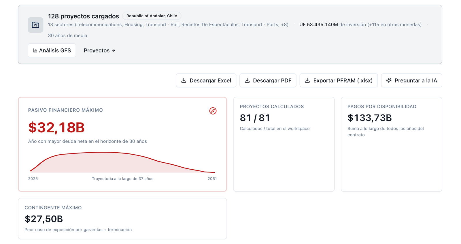
Figure 4.8 — FARO Overview: 81 / 81 contracts calculated; maximum financial liability $32.18B, maximum contingent $27.50B, availability payments $133.73B (the screen rounds to billions).

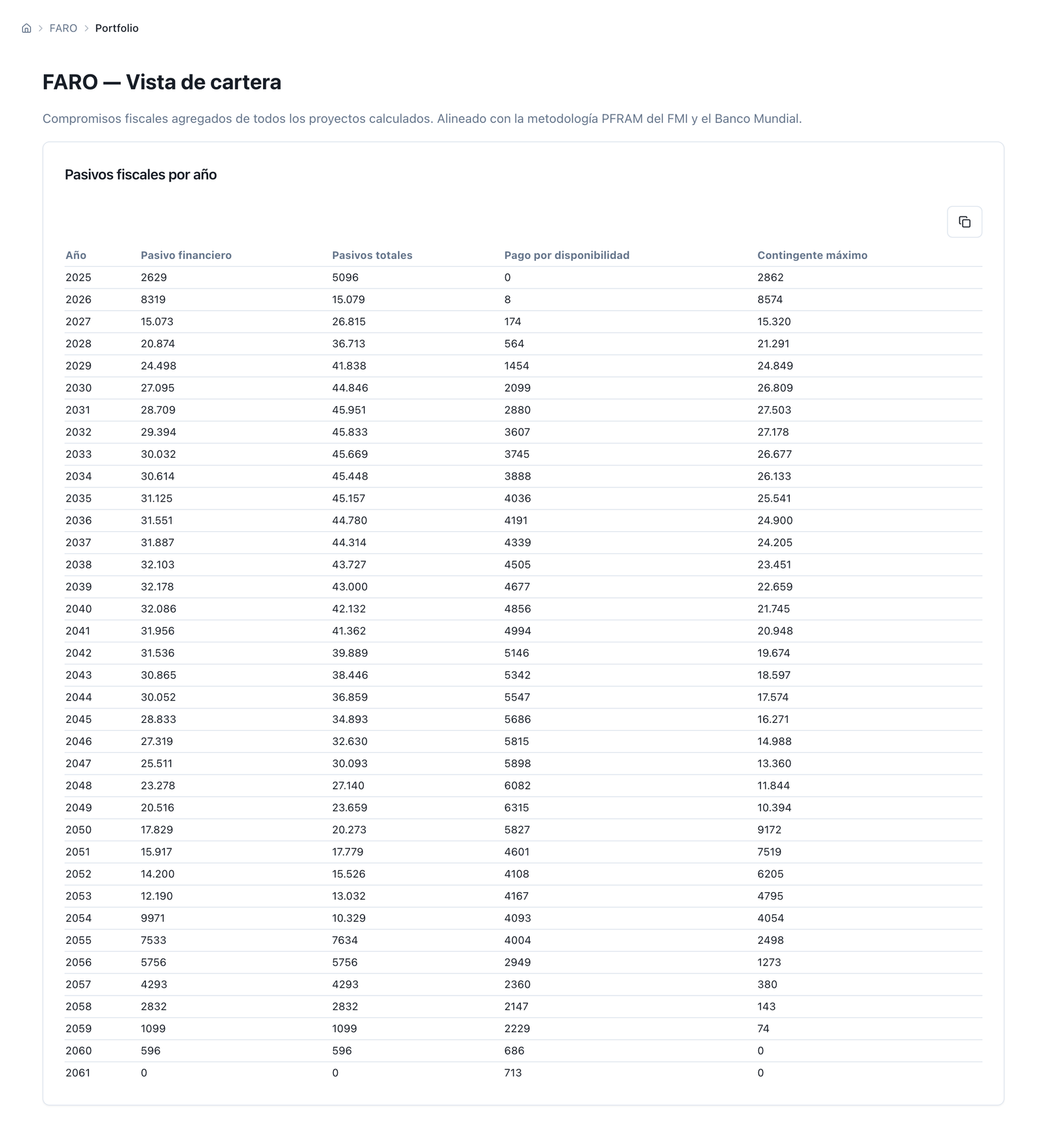
Figure 4.9 — Andolar's portfolio by year: peak total liabilities 45,951 (2031), financial liability 32,178 (2039), maximum contingent 27,503 (2031).

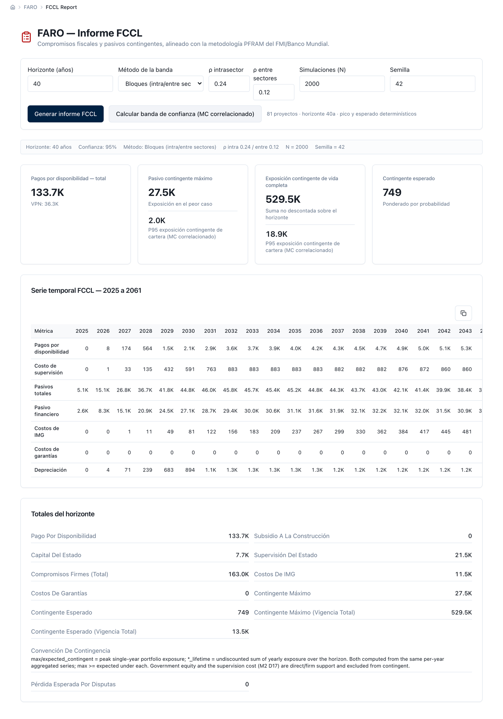
Figure 4.10 — FCCL report with horizon, band, N and seed now editable and printed: 40 years, blocks ρ 0.24/0.12, N 2,000, seed 42; maximum contingent 27,502.6 (27.5K), expected 749, lifetime 529,459.5 (529.5K) / 13,458.7 (13.5K), peak band 1,985.2 (2.0K) with the convention note printed. Only the lifetime band (18,900.0) has no card of its own.

The four figures for the contingent liability under its two conventions: peak maximum 27,502.6, peak expectation 748.9, lifetime maximum 529,459.5, lifetime expectation 13,458.7 (= 11,517.8 of MRG plus 1,940.8 of the greater of debt and termination; the three rows summed would give 14,441.3). Maximum ≥ expectation under each convention, because both are read from the same annual series. The sum of the per-contract peaks is 28,737.3, 4 % more than the portfolio peak, because not every contract reaches its maximum in the same year; in portfolios with more scattered schedules the difference is larger. The portfolio's full firm commitments — availability, equity contribution and supervision — sum to 162,972 in lifetime terms and 49,713 at PV; supervision is the second-largest firm item after the availability payment, and it appears on no screen. Coastal Highway is 2.0 % of the portfolio maximum in its peak year, 2.1 % of the lifetime expectation and 1.2 % of availability payments: a medium-sized contract in a portfolio of 81.

The MRG book under the volatility table. The same table from 4.4.1, summed over the 38 contracts with an MRG:

From 5 % to 30 % the book changes 22.8 times over from a single assumption, with the portfolio and the contracts identical. (Under the now-superseded total base, the leverage measured on the same portfolio was 28.7 times; the current figure, with the default demand base, is this one.) The expected MRG is 86 % of the portfolio's expected contingent liability; the volatility assumption is, by a wide margin, the one that moves the figure Finance publishes the most.

The correlated confidence band. A portfolio's guarantees are not triggered independently: a recession lowers traffic on every road at once. The base method simulates the portfolio with block correlation — 0.24 between contracts in the same sector, 0.12 between sectors, the extremes of Basel's asset-correlation formula, §2.6 — and presents the independent sum as a bound:

(FCCL report with the confidence band: figure 4.10.)

The mean does not move with correlation (786 against 781, against the deterministic expectation of 748.9: the simulation reconciles with the register), but the tail does: the peak's P95 rises 10 % with block correlation and 76 % if everything moved together. The figure that goes into the fiscal risk statement as "contingent loss at 95 % confidence" is 1,985.2 in the peak year and 18,900.0 in lifetime sum; the independent figure, 1,800.5, is the lower bound. And one more figure, the one that answers the spreadsheet of §6.5: the sum of each contract's VaR 95, each in its own peak year, is 4,315.0 — more than double the portfolio's VaR — because it sums tails that do not coincide in time or in path. Neither the sum of VaRs nor the independent sum is the portfolio's VaR; the first overstates it and the second understates it. With 2,000 paths the tail figures carry a visible sampling error; the report publishes the seed, N and confidence interval, and the screen flags "degraded" when it lowers N to respond in time.

4.6 Step 7: accounting, statistics and budget, from the same register

The control test (IPSAS 32). The State controls what services the road provides, to whom and at what price, and keeps the asset at the end: the contract passes the control test and the asset (645.0 at the close of construction) enters the grantor's balance sheet with an offsetting liability. In a mixed contract that liability splits in two, and the split is the first figure the register produces: the part of the asset the State pays for with the availability payment — 45 % of the cost, as measured by the engine over the contract's life — is a financial liability (IPSAS 32's financial liability model, ¶18–19; the MRG alone would suffice to require it, ¶19(b), §2.4); the part users pay for with the toll — the remaining 55 % — is a non-financial liability under the grant of a right to the operator (¶24–26), a deferred income recognised as "tariff imputed to users" as the concessionaire collects. The platform's ESA classifier reaches the same place by another route — construction and availability risk with the private party, but demand shared, a majority debt guarantee on its tranche and termination compensation at book value — and puts it on the balance sheet of the State with high confidence.

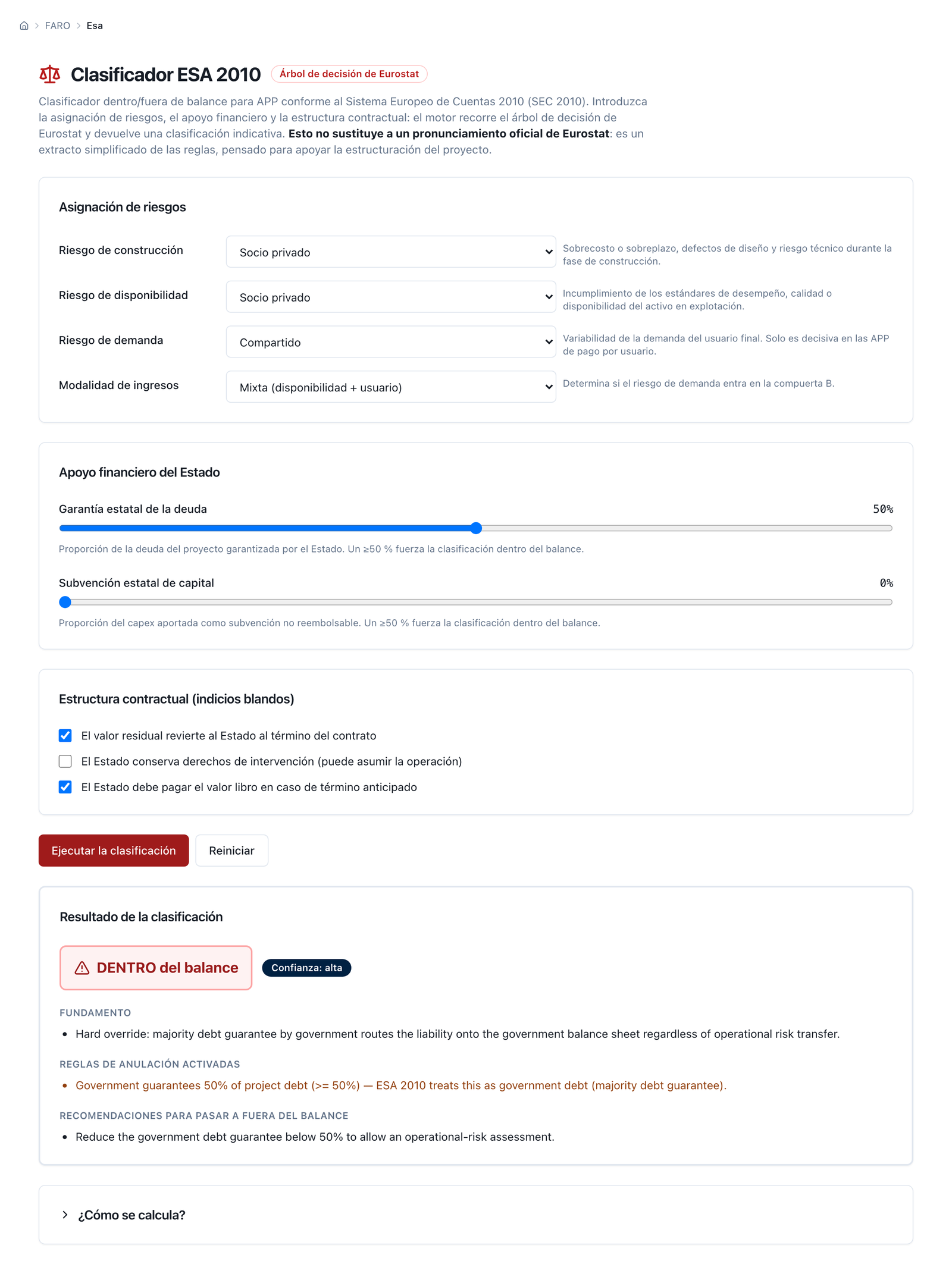
Figure 4.11 — ESA 2010 classifier on Coastal Highway: on balance sheet, high confidence — 50 % debt guarantee (≥ 50 %).

The two liabilities by year. The availability payment splits into finance charge, service expense and amortisation, at the rate that settles the financial liability over the contract's term (13.6 % effective, against 7.2 % on the loan: the availability payment pays a higher return than the debt); the liability under the grant of a right is reduced by the imputed tariff:

(Coastal Highway's FCCL, with the guarantee valuations and their reconciliation mark: figure 4.4.)

The financial liability is recognised during construction as the asset is built (110.0 → 307.6), keeps growing while the finance charge exceeds amortisation — peaking at 386.0 in 2039 — and is extinguished in 2052; the liability under the grant of a right is born with construction (368.6 in 2027) and is drawn down with the toll. The contract's total liabilities (financial plus grant of right) reach 676.2 at the close of construction, and the net loan is −239.5 in 2025: the State records the investment as its own in the year it is made, not when it pays for it. That is the recognition gap this manual attributes to Austral (§2.6): the budget will see 38.1 in 2028; the statistics saw 231.7 in 2025.

The IPSAS 19 note. Each valued guarantee is classified with the 0.5 threshold on the probability that it pays at least once in the contract's life (the annual figure goes into the note) and its expected cost at present value from the base year:

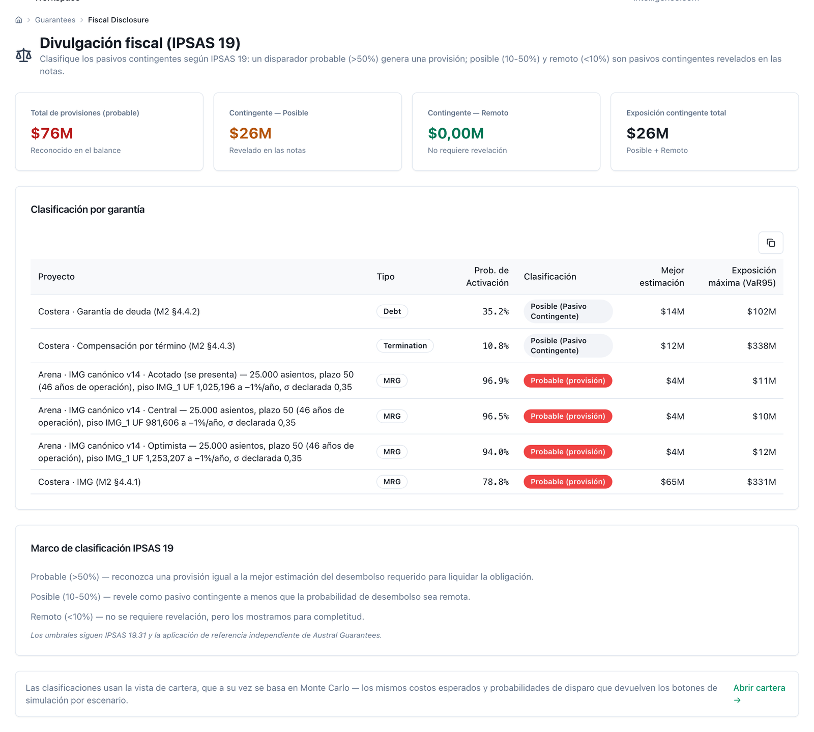
Figure 4.12 — IPSAS 19 note for Coastal Highway's three guarantees: 1 provision (MRG, 78.8 %), 2 disclosed contingent liabilities (35.2 / 10.8 %), best estimate 65 / 14 / 12, one currency.

One provision and two disclosed contingent liabilities, all in the same currency. The MRG crosses the threshold because, with the default demand base (§4.4.1), its lifetime probability jumps from 39.0 % (under the now-superseded total base) to 78.8 %; the register must declare the floor base it uses, because the entry depends on it. The debt guarantee's classification likewise follows directly from the annual probability: at the default 1.5 % its lifetime figure is 35 % and the guarantee goes to the note; at the 5 % the tool carried until September 2026 it was 76 % and the same clause was a provision of 37.1 at PV — the same contract, a different entry. In the portfolio, none of the 60 contracts with a debt guarantee crosses the threshold today (at 5 %, 59 of 60 crossed it), and with the default demand base the 38 of 38 MRGs cross it — before this correction, under the total base, only 21 did: those of the pure toll contracts, where the floor was already compared with the partner's whole revenue (4.4.1); the 17 mixed-contract MRGs, protected by the total-base artefact, now become provisions too. The register must declare the annual probability it uses and the MRG's floor base, because together they decide the entry. (The tool's note discounts the provision one period further, as a present-value approximation; the convention is unified in §5.)

The reconciliation. The three outputs of the same register, for this contract:

Ten figures for one obligation, and none is "the" figure. The IPSAS liability (386.0) is neither the budget commitment (1,546.1 of payments plus 322.5 of supervision) nor the augmented debt the statistics record (676.2) nor the contingent exposure (425.4): each answers a question, and all four reconciled on the same date from the same model. This is the table Step 7 requires as part of the report, and it is the one a register kept in three separate files loses (§6.6). The fiscal risk statement draws the contract's firm–contingent pair from here, and the GFS and IPSAS ledger screens show the same entries from their own statements.

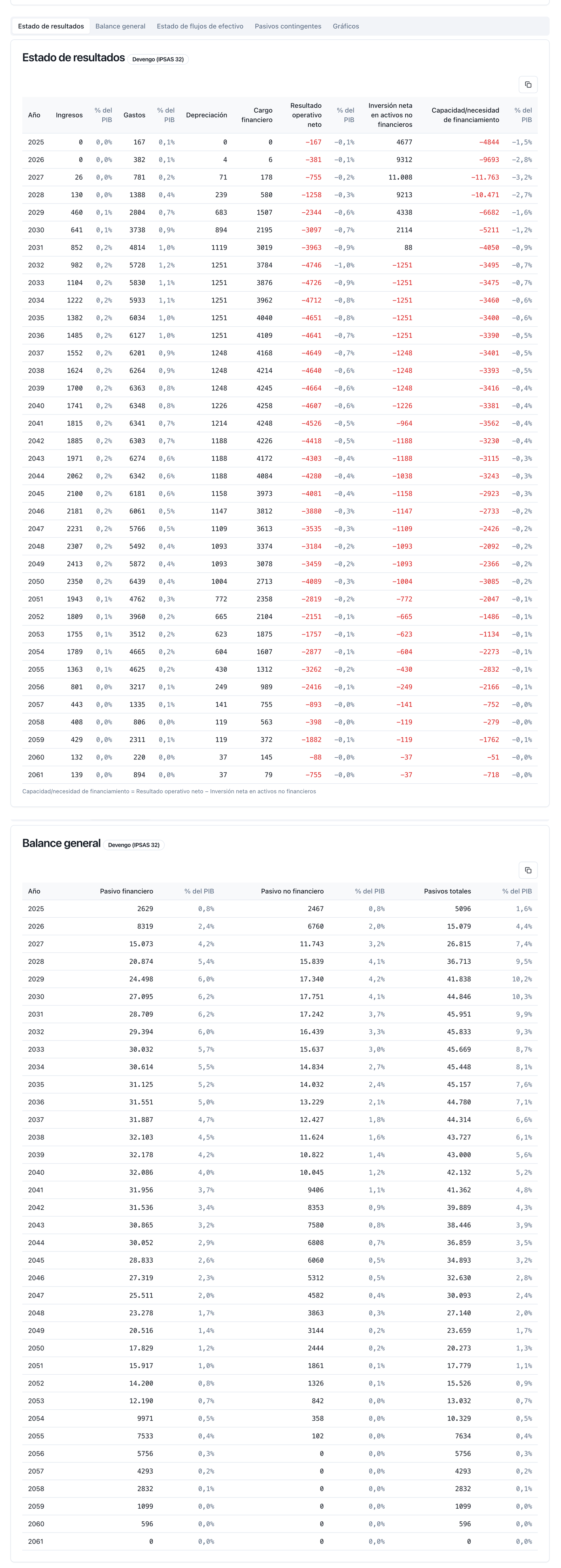
Figure 4.13 — The portfolio's GFS statements: statement of operations and balance sheet by year; total liabilities 45,951 in 2031 (9.9 % of GDP).

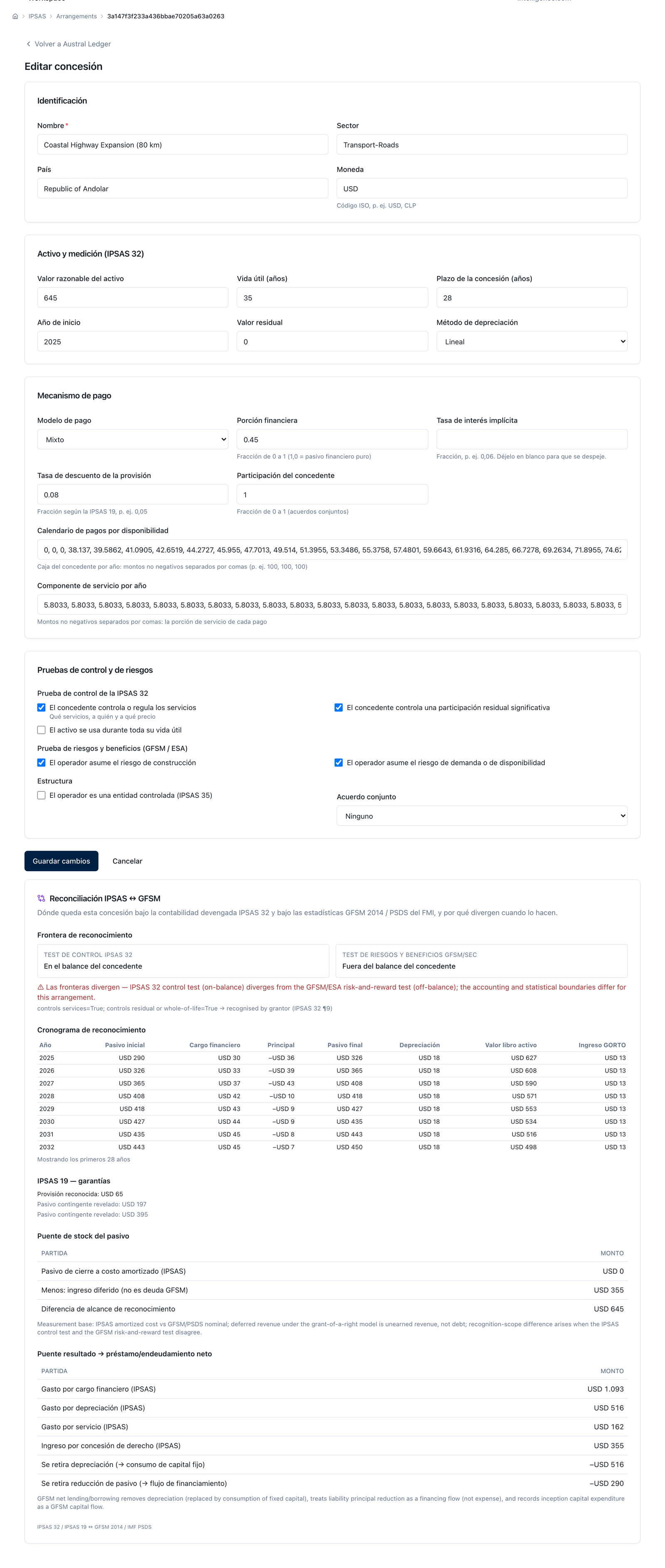
Figure 4.14 — Austral Ledger: Coastal Highway recognised on balance sheet (asset 645, liability 645, mixed model 45 / 55) with its year-by-year IPSAS 32 schedule and the IPSAS 19 note for the three guarantees: MRG as a recognised provision (65, the same PV as figure 4.12) and debt / termination as disclosed contingent liabilities (197 / 395, FARO's maximum exposure).

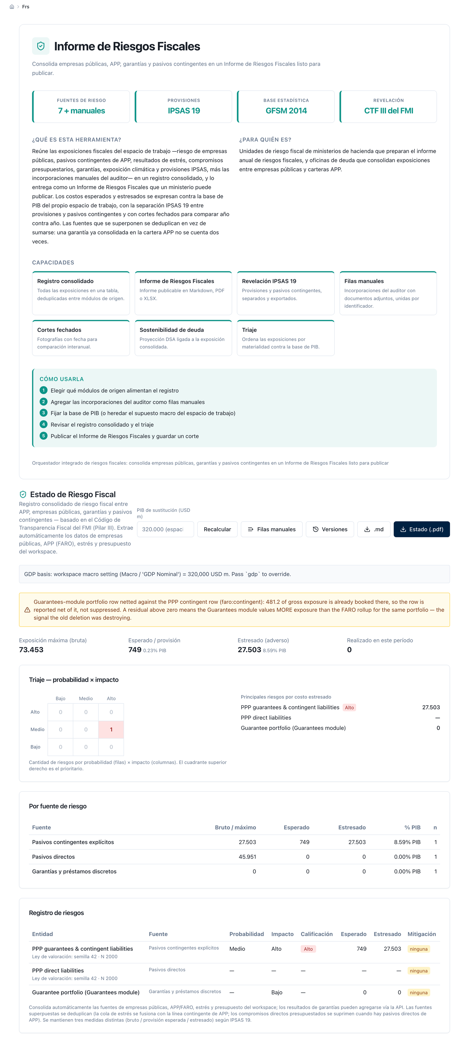
Figure 4.15 — Andolar's fiscal risk statement: the PPP portfolio as a firm (45,951) + contingent (749 expected / 27,503 maximum, 8.59 % of GDP) pair.

4.7 Step 8: the portfolio against the ceilings

The demo workspace sets two ceilings: firm commitments at 5 % of GDP and contingencies at 3 % of GDP, with an alert at 80 % of the ceiling. 2025 GDP is 320,000 and grows at 6.39 % nominal (2.5 % real plus 3.8 % inflation, the same price base as the indexed payments). Against the first ceiling the method scores the full firm commitments plus the full expected contingent liability — availability payment, subsidies, equity contribution and supervision, plus expected MRG, debt and termination under the exclusive rule — against the second, the maximum contingent liability. The Affordability screen already scores the full rule as its headline figure (exposure1_includes: availability payment, subsidies, equity contribution, supervision, expected MRG, debt and termination), with the earlier partial rule printed as a reference; supervision enters at its default value (2 % of investment per year of operation) with no need to declare it contract by contract, so the screen reproduces this section's 0.97 % of GDP exactly. The table carries both columns — the full rule and the now-superseded partial one — so that the screenshot reads clearly:

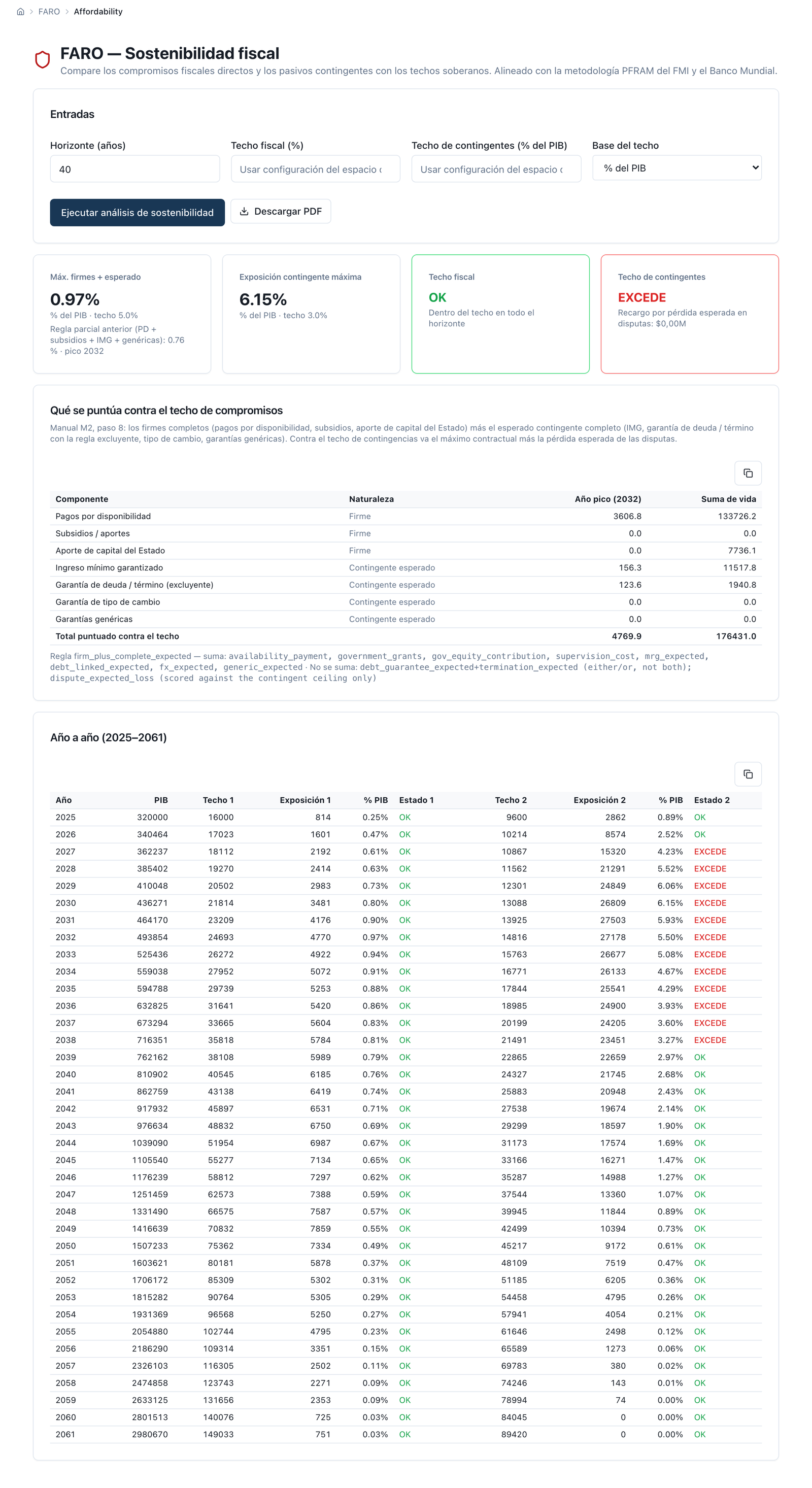
Figure 4.16 — Affordability: the screen scores full firm commitments + full expectation as the headline figure, 0.97 % of GDP in 2032 — reproducing this section's figure exactly, with supervision already included at its default value — with the earlier partial rule (0.76 %) printed as a reference; maximum contingent 6.15 % in 2030, EXCEEDS 2027–2038.

Full firm commitments plus expectation reach 0.97 % of GDP in 2032 — 19 % of the ceiling — and never touch it; in that year they consist of 3,607 of availability payments, 883 of supervision and 280 of expected contingent liability (the equity contribution has already ended). The earlier partial rule gave 0.76 % that same year: the difference, 0.21 pp, is almost entirely the portfolio's supervision (21,510 in lifetime sum), the firm item that rule did not score. The maximum contingent liability breaches the 3 % ceiling from 2027 to 2038, peaking at 6.15 % of GDP in 2030 (205 % of the ceiling), and stays on alert in 2026 and from 2039 to 2041 — the maximum, unlike the expectation, does not depend on the MRG floor base (4.4.4), so none of these figures moves because of that change. What the table teaches is not that Andolar is overexposed but what Step 8 says: a ceiling scored on the maximum is met by cutting guarantees, not by reducing risk. The same portfolio scored on the correlated CVaR 95 of the peak year (2,835.9: under 1 % of GDP even measured against 2025 GDP) sits well below it. Both rules are legitimate; the register declares which one applies (Austral, The Pipeline Under the Ceiling). And one more precision the screen already makes visible on its own: the full rule sums the expected equity contribution, supervision, debt and termination, all at their default value whenever the contract does not declare its own; the earlier partial rule, which left out supervision, is printed only as a historical reference. Coastal Highway alone weighs 0.010 % of 2028 GDP in availability payment, 0.014 % in full firm commitments plus expectation and 0.110 % in maximum contingent liability; the ceilings belong to the whole portfolio, not to the contract.

4.8 Steps 9 and 10: sensitivity, stress and versions

The contract's tornado (Step 9). Each bar is a full recalculation of the contract with one variable shocked in both directions, with the same random paths across all runs so the difference is the shock's, not chance's:

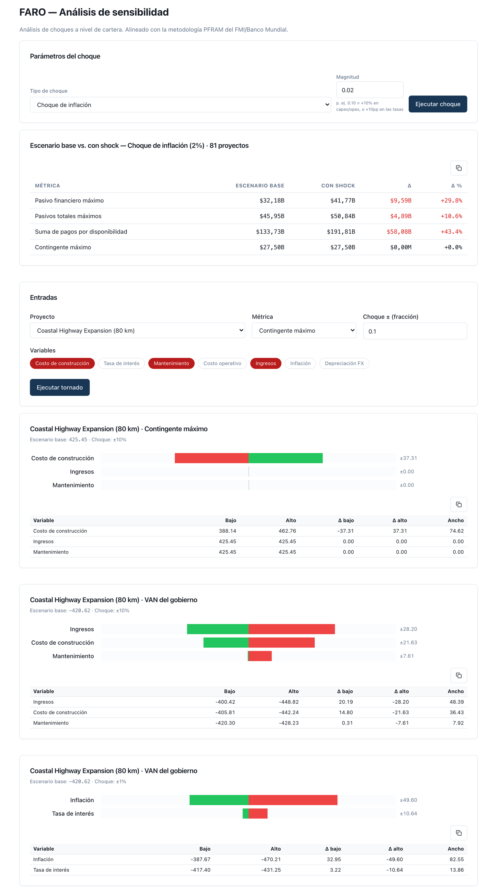
Figure 4.17 — Sensitivity and tornado: inflation +2 pp → payments +43.4 %, financial liability +29.8 %; Coastal Highway's tornado: construction 74.6 on maximum contingent; revenue 48.4, construction 36.4, maintenance 7.9 and, at ±1 pp, inflation 82.5 and rate 13.9 on the State's NPV.

On the maximum contingent liability only construction cost moves, because the maximum is a contractual stock — outstanding debt and the floor — and only debt depends on a tornado input; neither revenue nor inflation touches it. On the State's NPV (−420.6 in the base case) inflation (it indexes the availability payment) and revenue drive the result — and here the sign is surprising: higher revenue worsens the State's NPV, because the screen's revenue shock also scales the availability payment, which is a revenue for the partner and an expense for the State (the method defines the shock on user revenue; §5 declares it as a limitation). A discount-rate shock of ±2.5 pp leaves the maximum contingent liability at 425.4 on both sides and moves the State's NPV from −558.6 to −332.0: a stock is not discounted and the tornado does not report it. The screen applies a single magnitude to every variable; for rates, the example runs ±1 pp separately. The table's figures are those of the Tornado screen, which already computes the maximum-contingent metric too: its bars on maximum contingent (74.6 / 0.0 / 0.0) and on the State's NPV (36.4 / 48.4 / 7.9) match those of the engine against which annex 4.A checks them.

The portfolio shock. Inflation +2 pp across the 81 contracts:

(Sensitivity and tornado: figure 4.17.)

And a figure the table does not show, worth knowing: with 2 pp more inflation the portfolio's expected MRG falls from 11,518 to 5,741 (and the lifetime expected contingent liability, from 13,459 to 7,681), because tolls indexed to macro inflation pull away from floors whose indexation is contractual and fixed (3.8 %). An MRG protects against a fall in traffic, not against inflation; high inflation makes it cheaper and disinflation makes it more expensive.

The versioned register (Step 10). Four versions of the same contract, each with a cause, and the difference by cause:

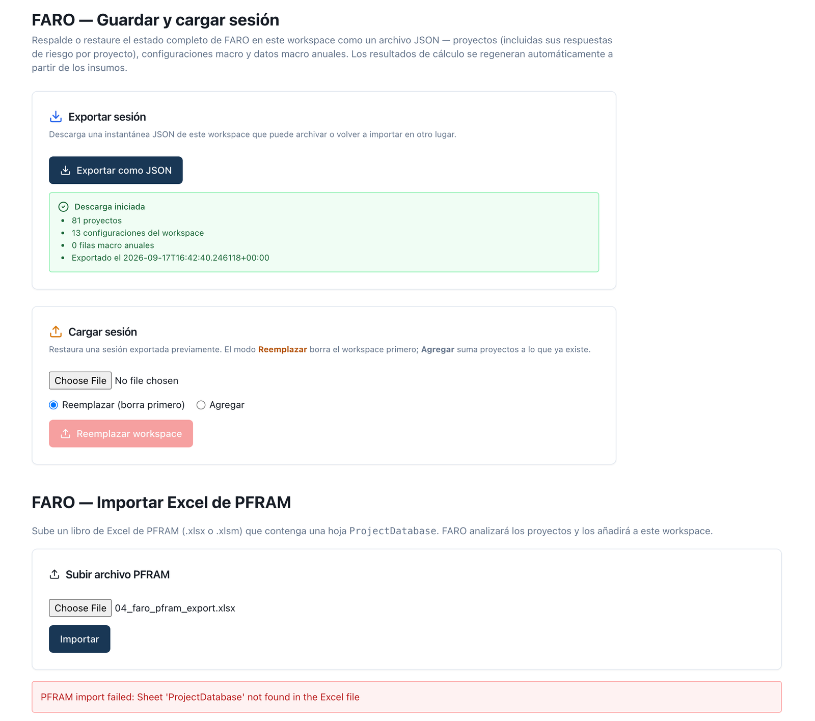
Figure 4.18 — Exported session (81 projects, 13 configurations, 2026-09-17) and the exported PFRAM workbook fed back into the importer, which replies "Sheet 'ProjectDatabase' not found".

Between v1 and v4 the expected contingent liability at PV is multiplied by 2.0 (79.9 → 163.4) and the firm commitment rises 32 %. Without the intermediate versions, next year's report would say "exposure went up" and nobody could separate what changed in the world (the refinancing: +0.6 on expected debt) from what changed in the analyst's head (volatility: +124.8) or in the rule (the rate: +222.4 on the firm total). And a fifth version, which this manual documents in annex 4.A: that of a change in one of the tool's default values (the guaranteed debt's annual probability, 5 → 1.5 %), which lowered expected debt from 62.5 to 26.4 without the contract or the analyst changing; and a sixth, documented in this same section: the change in the MRG's floor base (from "total" to the default "demand"), which raised the MRG's expectation from 68.0 to 254.8 without the contract, the analyst, or any declared assumption changing. The platform stores each version as a dated session; the table of changes by cause is built from two sessions, and that is what Step 10 requires to be published.

Box 4.9 — The user-pays corridor: when everything is contingent. The Northern Road Corridor (120 km, US$ 895 M, 30 years, maximum debt 671.2) pays for itself with tolls linked to GDP. The State pays the concessionaire nothing: no availability payment, no equity contribution. Its only firm commitment is supervision (17.9 a year over 26 years of operation: 465.4 in lifetime sum, 153.6 at PV), which exists even in the contract that costs the budget nothing, and which is exactly why it belongs in the register. What it does have is the MRG (peak floor 66.1; expectation 98.9 in lifetime sum, with a 63 % call probability, because here the floor is 80 % of the partner's whole revenue: a provision under IPSAS 19, not a note) and the termination compensation (maximum 671.2; expectation 42.4). Peak maximum contingent liability 687.4 in 2029 and lifetime expectation 141.3, against a positive State NPV of 34.7 from the company's taxes. In the register this contract is the mirror image of Coastal Highway: almost nothing in the budget, everything in the memorandum item; and in the 5 % ceiling it weighs only its supervision, while in the 3 % ceiling it weighs 2.5 % of the portfolio. A ministry that only looks at firm commitments does not see it.

Box 4.10 — The availability hospital: all firm, plus debt. The Central University Hospital (800 beds, US$ 690 M, 30 years, a 25 % equity contribution: 172.5) is the other extreme: an availability payment of 93.0 in 2029 growing to 236.2, 4,006.1 in lifetime sum and 1,130.9 at PV; firm commitments with the contribution and supervision (13.8 a year; 358.8 in lifetime sum, 118.4 at PV), 1,404.6 at PV and 4,537.4 in lifetime sum. It has no MRG — there is no revenue to guarantee — and does have a debt guarantee (maximum 181.1, expectation 25.6, lifetime probability 35.0 %: to the note, as with Coastal Highway) and termination (362.2 / 22.6). Peak maximum contingent liability 362.2 in 2028, lifetime expectation 27.0. State NPV −1,116.3. It is the M1 contract seen from the other side: what there was "the cost of the PPP" is here a thirty-year firm commitment in the medium-term framework, and its contingent liability is small and debt-driven. The two boxes show why the register needs both lists: in the hospital what matters is the firm commitment; in the corridor, the contingent liability; and in Coastal Highway, both.

Box 4.11 — Chilean practice: how an MRG clause reads in a real contract, and how Dipres reports it. In the tender documents for the Puente Industrial road concession (MOP, 2013), the demand-risk-sharing mechanism sits in article 1.12.7.1: the State guarantees, for each calendar year of operation, a minimum revenue (Y^min) set in Table No. 7, in UF, between operating years 1 and 16 (Clarifying Circular No. 3, answer 30), and pays the difference whenever toll revenue falls short. The clause has the four pieces Step 3 asks one to read: the floor (a table by year, not a percentage), its indexation (it is in UF: full inflation), its window (16 years, not the contract's term) and its price: under article 1.12.2.1.2 the company pays MOP UF 48,000 in two instalments for the guarantee, and may waive it by certified letter up to 180 days before each instalment, upon which "the obligations of the State and of the Concessionaire" regarding the mechanism are extinguished. The contract is also structured on a present value of revenue (VPI) basis: any MRG payments the State makes are deducted from the accumulated VPI, so the guarantee advances revenue and extends the term rather than giving it away outright. A register that reads only "MRG: yes" loses all four things. The El Loa airport's first concession (tender documents, art. 1.14.2) is the other pattern: an annual MRG table with a 50 % revenue-sharing rule for the State above a threshold — floor and cap in the same clause. Dipres reports these guarantees every year in its Informe de Pasivos Contingentes (Contingent Liabilities Report; an obligation under article 40 of DL 1.263, with the paragraphs added by Ley 20.128), and its structure is the one Step 7.1 proposes for the PPP chapter of a fiscal risk statement: for each mechanism, the nature and the beneficiaries, the maximum exposure, the expected value — for the MRG, by simulating traffic revenue in two stages, §II.3.3 and §III.2 of the 2025 edition — and the year's payments. This manual cites its structure, not its figures.

4.12 What Finance would do with this result

Finance has in front of it, for Coastal Highway, a firm commitment of 697.8 at PV (1,965.4 nominal: 51.0 → 106.2 per year, of which 12.9 is supervision), a maximum contingent liability of 425.4 in 2028, an expected contingent liability of 283.0 in lifetime sum (79.9 at PV) and an IPSAS 19 note with one provision (the MRG) and two disclosures; and for the portfolio, 81 contracts that fit comfortably under the firm ceiling (19 % under the method's rule) and do not fit under the contingencies ceiling when scored on the maximum. With that, the sensible course is to register and approve the contract with four conditions, not to simply "note" it:

1. Write down the volatility and the default probability with a name and a source. The two default figures (15 % and 1.5 %) between them decide 100 % of the MRG's expectation and the debt guarantee's accounting entry. At 10 % and 1.5 % the contract would have 131.2 of MRG and 26.4 of expected debt; at 20 % and 5 %, 379.6 and 62.5, and the debt would also be a provision. Neither is more true; the one in the register has to be someone's.
2. Declare the MRG's floor base in the mixed contract. Floor compared with the demand revenue the guarantee insures, not with the availability payment that can never trigger it: 254.8, the platform's default value. Write it into the profile, because the same floor compared with total revenue would give a different guarantee — and it is, in fact, the one this manual published (68.0), until it was identified as an artefact of the bridge between FARO and the guarantees engine.
3. Score the ceiling with a stated rule. On the maximum, the portfolio breaches the contingencies ceiling for twelve years; with full firm commitments plus expectation against the 5 % ceiling, it sits at 19 %; with the correlated CVaR 95 of the peak year against the 3 % ceiling, well under a third. Coastal Highway does not change the verdict under any of them; the verdict depends on the rule, and the rule is a decision for the Ministry.
4. Fix the version. The contract profile with a date, seed, N and the six assumptions (rate, volatility, PD, recovery, termination probability, ρ) is this year's register; next year's is compared against it cause by cause.

What Finance would not do: add 197.4 and 394.7 together as the contract's "exposure" (the debt is counted once); count the 96.8 of equity contribution as contingent; leave the 322.5 of supervision out of the register because it is not paid to the concessionaire; report "MRG: no expected cost" because the base path does not touch it; or present 1,985.2 as "the loss" of the portfolio without saying it is a correlated 95th percentile with a declared ρ.

Annex 4.A — How to reproduce it in three steps in the guest workspace

1. Load the portfolio. Enter the platform without registering — a guest workspace is created — and open FARO. If the demo portfolio is not loaded, load it from the home screen (81 contracts from the Republic of Andolar, with the example's macro assumptions and ceilings). Open Projects and the Coastal Highway Expansion (80 km) contract: the Government and Guarantees tabs show the profile from 4.1 (indexed toll and availability payment, floor 37.31, volatility 15 %, 50 % coverage with a 1.5 % annual PD and 40 % recovery, 10 % cumulative termination). If the portfolio was loaded before September 2026, reload it: the guaranteed debt's probability was saved as an explicit value on each contract (5 % in earlier loads), so Calculate all keeps it as is; only the reloaded package seeds the current 1.5 %.
2. Read the contract. On the contract's FCCL tab: availability payment 38.1 → 93.3, peak financial liability 386.0, peak maximum contingent liability 425.4 and expected 283.0 in lifetime sum, with the "3 of 3" reconciliation mark against the guarantee tools. In the Guarantees module → MRG, Debt, Termination, load the same parameters (the FCCL tab publishes them, with the "demand" floor base it declares by default) and run with seed 42 and 2,000 paths: MRG 254.8, debt 26.4, termination 24.5, with their VaR and CVaR. Supervision (12.9 a year from 2028 to 2052) is already in the firm-commitments schedule: the Costs tab brings it in at its default value, 2 % of total investment per year of operation.
3. Read the portfolio. FCCL Report: peak 27,502.6 / 748.9, lifetime 529,459.5 / 13,458.7, PV of availability payments 36,321.9 at 8 %; click confidence band with block correlation: peak P95 1,985.2, lifetime 18,900.0, N 2,000, seed 42, not degraded. Affordability: 0.97 % / 6.15 % of GDP under the full rule the screen already scores and reproduces exactly (0.76 % is the earlier partial rule, printed only as a reference), contingent ceiling breach 2027–2038. Sensitivity: inflation +2 pp → availability payments +43.4 %. Tornado on the maximum contingent liability: construction cost ±10 % → width 74.6; on the State's NPV, 36.4.

Assumptions the example adds and declares. The five ratings in the 4.2 matrix are the text's own; the demo portfolio ships the matrix unassessed. Supervision is already modelled by the tool at its default value (2 % of total nominal investment per year of operation), in the contract and in the portfolio. The four versions in 4.8 are built by editing the contract (volatility, loan rate) and the workspace's rate. The platform stores sessions, not the causes table. The example's policy rate is the workspace's (8 %) and the figures at 5.5 % are obtained by changing it and recalculating. A verification script reproduces every figure in this section from the engine and checks it against the workspace via the API: in the 17-09-2026 run every contract and portfolio figure matches, including the tornado bars on the maximum contingent liability, the IPSAS 19 note and Affordability's full rule.

Version note: the figures before and after the change in the default probability and in supervision as a firm commitment. The first version of this section (16-09-2026) was calculated with the annual default probability on the guaranteed debt the tool carried by default, 5 %, and without supervision among the firm commitments. The 1.5 % went into production on 16-09-2026 and supervision was decided the same day; this version (17-09-2026) recalculates everything with both. Nothing else changed: same portfolio, same seed, same N, same volatility, same recovery, same rate. Both columns are kept because a register must be able to explain, figure by figure, what changed and why (Step 10):

5. Implementation on the Austral platform

The method of section 3 can be run with any tool. This section describes how the two Austral modules that share it run it: FARO —the Fiscal Risk and Obligations Assessment register, aligned with PFRAM 2.0— and Guarantees —the Guarantee and Contingent Liability Valuation workshop, where each guarantee is designed and valued—. For each screen: which step it runs, what input it asks for, what output it delivers, what the analyst decides and where the limit is. The screenshots are from the guest workspace with the demonstration portfolio of the Republic of Andolar and the contract of section 4 —never client data— and are numbered in the order of the method, not of the menu. Everything that follows exists today; where a capability is not implemented, it is said.

5.1 Where the modules live and how to get in

FARO lives at platform.austral-intelligence.com/workspaces/<workspace>/faro and Guarantees at …/guarantees; every screen is a route under those addresses (…/faro/fccl-report, …/guarantees/mrg, …/faro/projects/<contract>/fccl), so a record is shared by sending a link. No registration is needed to try it: on entering, a guest workspace is created with its own database, which is kept if it is later converted into an account.

The demonstration portfolio —81 Andolar contracts, with the macro assumptions (inflation 3.8 %, growth 2.5 %, exchange rate +2 %/year, GDP 320,000), the workspace's policy rate (8 %) and the two ceilings (5 % and 3 % of GDP, alert at 80 %) of section 4— is loaded from the FARO home screen. Two things worth knowing before pressing it. Loading the pack adds the 81 contracts to any already in the workspace —loading it twice duplicates them— and overwrites the workspace's macro assumptions and ceilings with the demo's; the workspace reset, which does delete everything, requires confirmation. And each contract's results are cached with a fingerprint of its inputs, of the macro assumptions and of the engine version that computed them: when an input changes, the contract recalculates on its own, and when what changes is the engine —a valuation rule, a default value— the contract recalculates on its own when it is read, with no need to press Calculate all; the register records, in each version, which engine version it was calculated with.

Two points of form, as in M1. The two modules' screens are labelled in English today —the text gives in parentheses the name the manual uses—, while navigation, the downloadable reports and the help sheets are in Spanish, English, French and Portuguese. And each module ships its own online methodology page (Manual in FARO, Methodology in Guarantees): this manual is its extended version, not its replacement.

5.2 Screen‑by‑screen walkthrough — FARO, the portfolio register

Steps 0 and 6 — Overview

Label: Overview. Input: none; it reads the workspace contracts' cached results. Output: the portfolio indicators —contracts loaded and calculated, financial liability in its peak year, total liabilities at their peak, lifetime sum of availability payments, maximum contingent liability at its peak, with and without disputes—, rounded to billions by card convention (the one‑decimal figures are in Portfolio and in the report), and the annual chart of the series. Analyst's decision: none here; it is the Step 6 dashboard. Limit: the overview reads only the cache; a contract that is loaded but not calculated counts in "contracts" and not in "calculated", and the gap between the two numbers is the first thing a reviewer should check. The top strip of "projects loaded" counts every row in the workspace —from every module, not only the FARO portfolio— and mixes currencies.

(Andolar portfolio overview: figure 4.8.)

Steps 1 and 2 — Projects and the contract profile

Label: Projects and, within each contract, the tabs Assets, Revenues, Costs, Government, Financing, Private Partner, Guarantees, Risk, Results and FCCL (fiscal commitments and contingent liabilities, FCCL). Input: the Step 1 profile —assets with their investment, schedule and useful life; in Revenues, the availability payment and the toll, by type (user‑pays, availability, mixed) with their indexations; in Costs, the concessionaire's maintenance and the State's supervision cost, at its default value (2 % of the investment per year of operation) with a provenance mark that distinguishes the default value from the one declared by the contract; in Financing, the debt tranches with rate, tenor, grace period, amortisation, currency and the State's equity stake; in Private Partner, the equity and the tax—. The Government tab is not the input sheet: in production it shows the contract's GFS statements for the State (net lending, financial liability, contingent liability), not the three cards above; the inputs section 4.1 attributes to it live in Costs, Financing and Revenues. Output: the contract's cash‑flow model, which runs on saving and feeds every other tab; and, in the list, each contract with its sector, its mechanism and its calculation status. Analyst's decision: the whole contract model; the source can be this profile, the imported PFRAM workbook (screen 12) or the transfer from the Contract Registry (section 5.5). Limit: the equity contribution is not typed in: it is derived from the stake × each construction year's investment, as Step 2 requires, and appears in the Government grants / equity series of the result. The profile has no signed / in tender / pipeline tag from Step 0: every contract in the workspace is added up as a single portfolio, so FARO loads only signed contracts —the ones the method values— and the inventory of contracts in tender and in the project pipeline is kept in the report's table, outside the tool.

(Coastal Highway contract profile: figure 4.1.)

Step 3 — The contract's Guarantees tab

Label: Guarantees, within the contract. Input: four cards, each with exactly the keys the valuation engine reads, at their default values. Minimum revenue guarantee (MRG): enable; floor shape (indexed base floor, price × demand, or a year‑by‑year table); floor base (demand revenue, by default, or declared total revenue); guaranteed price and demand; floor indexation and growth of guaranteed demand; window (first and last contract year); revenue volatility, with no default value —if left blank, the engine values it at 15 % and the report flags it as undeclared—. Debt guarantee: coverage of outstanding debt (0 = no guarantee); default probability, labelled annual; recovery after default, also with no default value. Termination: enable; cause (concessionaire, State, force majeure); compensation base in the engine's vocabulary (book value of assets, outstanding debt, fair value, fixed amount, PV of remaining flows —the cause decides the formula, except with a fixed amount—); probability, labelled cumulative over the contract; fraction of lost return (only with State cause); year of single exposure. Exchange rate: enable; base rate, guaranteed depreciation threshold, volatility, domestic and foreign rates, notional (blank = investment × imported components); it does not ask for a probability, because the engine derives it from the exchange‑rate process. The button saves and recalculates. Output: the four valuable rows of the Step 3 contingency register, with the assumptions Step 5 will use. Analyst's decision: reading the clauses and the declared assumptions; the MRG's call probability is no longer asked for, because under simulation it is endogenous to the revenue distribution and asking for it counted it twice. Limit: a contract saved with the tab as it was before this fix keeps its old keys with no effect on the engine (the profile lists them at the foot, e.g. mrg_coverage_pct, debt_guarantee_enabled); the migration proposes the equivalent value only where the engine's key is blank, and deletes nothing.

(Coastal Highway guarantees: figure 4.2.)

Step 3.1 — The Risk tab

Labels: Risk (risk matrix), within the contract; and Risk Matrix at portfolio level. Input: PFRAM's eleven categories with their questions; per category, likelihood and impact on five levels (1–5, not three) whose product the platform groups into four bands (Low 1–3, Medium 4–7, High 8–14, Critical 15–25), mitigation and priority. Output: the rating on the 5×5 matrix, the band and the priority of each category, and the associated exposure metrics; at portfolio level, the map of ratings by contract. Analyst's decision: each rating is their own judgement, with its line of support; the tool infers none of it from the financial data. Limit: the matrix does not produce figures that enter the register (Step 3.1); and the demo portfolio carries it unevaluated: the five rows of section 4.2 are loaded by hand into the workspace before screen 4 is captured, and the figure says so.

(Coastal Highway risk matrix: figure 4.3.)

Steps 4, 5 and 7 — The contract's FCCL tab

Label: FCCL, within the contract. Input: the calculated contract. Output: the contract summary; the private branch's viability (debt service coverage, IRR); the annual FCCL schedule —availability payment, financial liability with its split into financing charge, service and amortisation, maximum and expected contingent liability, total liabilities—; the guarantees with their peak (MRG, debt, termination) and their valuation law; the reconciliation mark with the guarantee tools (each guarantee re‑valued by the workshop with the same parameters reproduces the register's series bit by bit): a "Matches the Guarantees module" chip and a ✓ column per row —not a printed "3 of 3" counter—; and the export to text and print. Analyst's decision: reading each guarantee's three figures and checking that the reconciliation closes before moving on to the portfolio. Limit: the schedule applies the exclusive debt/termination rule to the contract's maximum and expected figures (Step 5), but the IPSAS 19 note is not assembled here (screen 21); the present value of the expected figure is discounted from the base year throughout the block —the method's convention (Step 7), now a single one across the register, the workshop and the note—.

(Coastal Highway FCCL: figure 4.4.)

Step 6 — Portfolio

Label: Portfolio. Input: the cached results. Output: four aggregated portfolio series by year —financial liability, total liabilities, availability payment and maximum contingent liability—, in a table; there is no chart on this screen. Analyst's decision: none; it is the Step 6 sum before it is summarised. Limit: the portfolio is the whole workspace; there is no filter by the Step 0 tag. The series with GFS‑statement keys (revenue, expense, net lending, non‑financial assets, net worth) and their chart are not here: they live in GFS Statements (section 5.4).

(Andolar portfolio, aggregated series: figure 4.9.)

Step 6 — FCCL Report and the confidence band

Label: FCCL Report. Input: the horizon and, for the band, the correlation method (a single ρ, sector blocks, a matrix, a GDP factor), the ρ values, the confidence level, N and the seed. Output: the portfolio totals —availability payments, subsidies, equity contribution as a direct commitment, MRG, guarantees—; the maximum and expected contingent liability under both conventions, annual peak and lifetime sum, with the convention note printed; the present value at the workspace rate; the series; and, on pressing the band, the correlated Monte Carlo block: method, ρ with its cited basis, N, seed, P50 / confidence percentile / mean by year, peak and lifetime sum, VaR and CVaR, the reconciliation of the mean with the deterministic expected figure, and the degraded mark if the tool lowered N to respond in time. Analyst's decision: the correlation structure —the manual's base method is 0.24 / 0.12 blocks— and the confidence level; horizon, method, ρ, N and seed are already editable fields on the screen, with the method's values as the default. Limit: the band is for the whole portfolio, not by contract; the VaR breakdown by contract belongs to the workshop (screen 19, not included) and to the API. The band card only prints the peak percentile; the lifetime one (15,643.3) is returned by the API (mc_band.lifetime.p_conf) with no card of its own on screen.

(FCCL report with confidence band: figure 4.10.)

Step 8 — Fiscal Affordability

Label: Fiscal Affordability. Input: the two ceilings (% of GDP or of revenue, and % of GDP), the base, the alert threshold and the horizon; the workspace saves them and the screen prefills them. Output: GDP projected at the workspace's nominal rate; by year, exposure against each ceiling in money, in % of GDP and in % of the ceiling; the breach years and the alert years; and its own PDF. Analyst's decision: the ceilings and the threshold, which are fiscal policy, not model output; and the reading of the rule. Output (full rule): the screen scores against the first ceiling the full Step 8 rule —availability payment + subsidies + equity contribution + supervision + expected MRG, debt and termination under the exclusive rule—, with the breakdown printed row by row and the earlier partial rule cited only as a reference; against the second, the maximum contingent liability plus the disputes' expected loss. Supervision enters at its default value without the contract having to declare it, so the screen reproduces exactly the figure in section 4.7.

(Andolar affordability: figure 4.16.)

Step 9 — Sensitivity and Tornado

Labels: Sensitivity (portfolio sensitivity) and Tornado Sensitivity (tornado by contract). Input: on the first, the type of shock —construction cost, operating costs, inflation, exchange rate or compound macro shock— and its magnitude, over the portfolio; on the second, a contract, the metric (project NPV, State NPV, IRR, maximum debt, maximum contingent liability, mean coverage), the seven variables the screen offers (construction cost, interest rate, maintenance, operating cost, revenue, inflation, exchange‑rate depreciation) and the shock's magnitude, a single one for all of them. The discount rate is not on the list: the ±2.5 pp shock section 4.8 uses cannot be run from this screen. Output: the base / shock / delta table of each portfolio series, and the tornado with the bars sorted. Analyst's decision: the metric —the one the ceiling scores— and the variables. Limit: the screen's "revenue" shock also scales the availability payment, so in a mixed contract more revenue worsens the State's NPV: the method defines that shock on user revenue (Step 9), and as long as the screen does not separate them, the revenue bar of a mixed contract reads as a shock to the private partner's total revenue and the availability‑payment shock is read on the inflation bar. A discount‑rate shock on a stock gives zero and is not reported; and the single magnitude forces the rates to be run separately (section 4.8 uses ±1 pp).

(Portfolio sensitivity and Coastal Highway tornado: figure 4.17.)

Step 7 — ESA 2010 Classifier

Label: ESA 2010 Classifier. Input: Eurostat's European System of Accounts 2010 (ESA 2010) decision tree —construction risk, availability risk, demand risk; public financing; guarantees; termination clauses—, shared with the Value for Money module. Output: on‑ or off‑balance‑sheet for the State, with the confidence level and the reasons. Analyst's decision: each answer on the tree. Limit: the classifier itself warns that it is a simplified extract of the rules and does not substitute for an official ruling; it is Step 7's second opinion, alongside the IPSAS 32 control test the FCCL tab applies.

(ESA 2010 classifier on the Coastal Highway: figure 4.11.)

Steps 1 and 10 — Import PFRAM and Save & Load Session

Labels: Import PFRAM and Save & Load Session (Session). Input: a contract's official PFRAM 2.0 workbook (ProjectDatabase sheet); and the workspace's JSON session. Output: the contract imported as a Step 1 profile, with a report of which fields were read and which were skipped; the export back to PFRAM format; and the session —contracts, macro assumptions, ceilings, results— as a single file that is downloaded and loaded again, which is Step 10's version. In addition, every contract admits branches and versions with an input diff between two versions, from the workspace's project list (…/projects/<contract>/versions). Analyst's decision: the date and the name of each version. Limit: the platform saves versions and shows the input diff; the by‑cause diff table of section 4.8 is assembled from two versions, by hand. The fiscal risk statement has its own "vintages" with a diff between two, at portfolio level. The flat PFRAM format does not round‑trip through this screen: "Export PFRAM (.xlsx)" writes the flat format (Cover, Macro Inputs, Project List, Cash Flows…), but Import PFRAM Excel only accepts the official ProjectDatabase sheet and returns an error with the flat format; the flat‑format importer exists in the API (POST /faro/import/pfram-flat) but has no screen of its own.

(Exported session and Coastal Highway PFRAM workbook: figure 4.18.)

Section 6 audit — FARO exports

Label: the report's download buttons. Output: an Excel workbook —the portfolio's fiscal liabilities; the FCCL table; the contract inventory; sensitivity, if it was run; guarantee assumptions, with the volatility used by each MRG, its provenance (declared or undeclared reference value) and the 5/10/15/20/30 % sensitivity table, and the valuation law, seed and N of each guarantee; and depreciation by asset— and a PDF —cover page, portfolio summary with indicators and series, detail by contract, and fiscal impact with the two ceilings and their breaches—. Limit: the PDF does not carry the confidence band or Step 7's reconciliation table: the band is taken from the on‑screen report and the reconciliation is assembled by hand between FARO, GFS and the ledger (section 5.4).

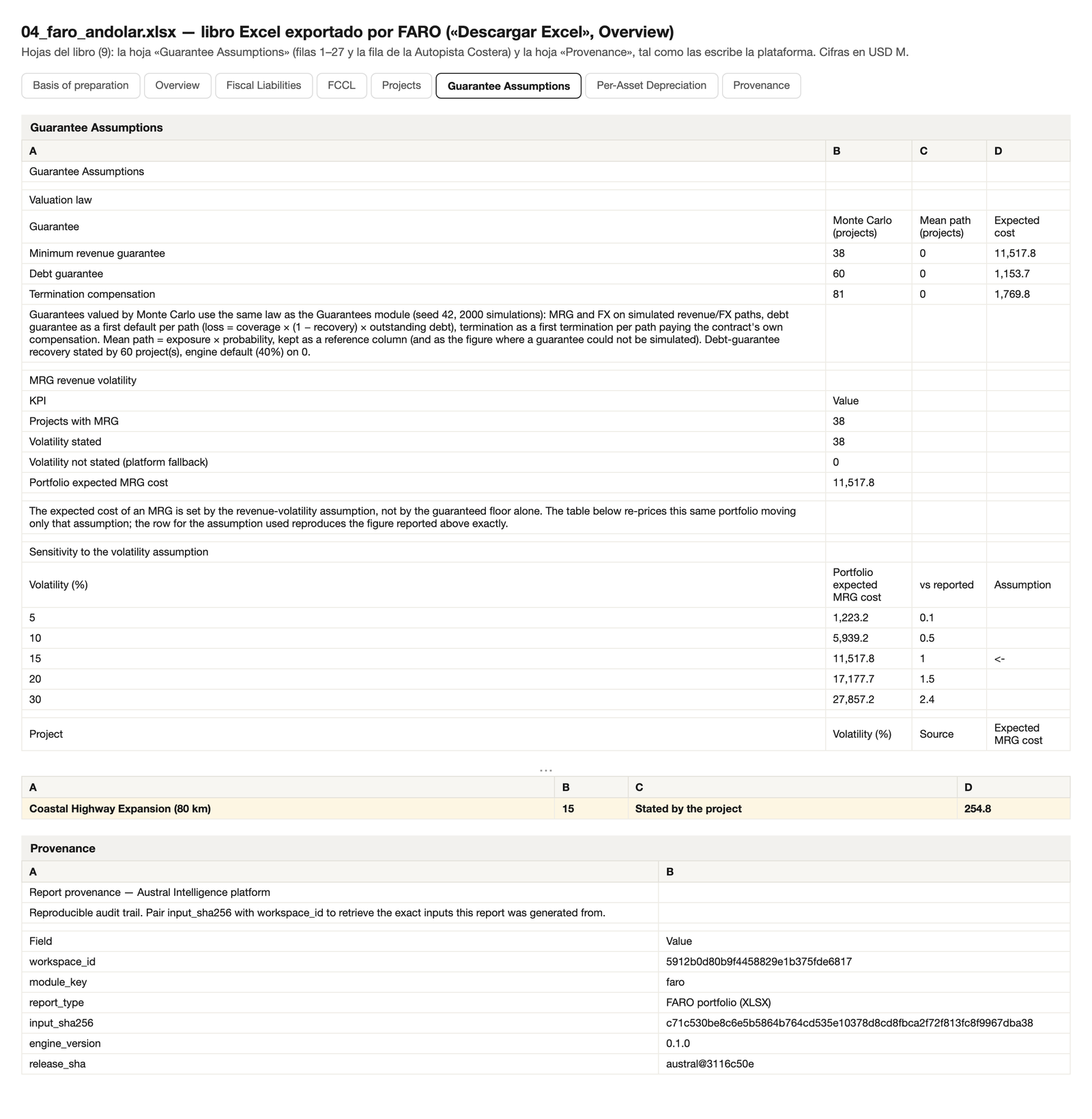
Figure 5.12 — "Guarantee assumptions" sheet of the Excel workbook: the declared 15 % volatility of the Coastal Highway's MRG and its table 27.0 / 131.2 / 254.8 / 379.6 / 614.3 (section 4.4.1); the valuation law, seed 42, N 2,000 and the floor base ("demand", by default) of the three guarantees.

Named in a single line, with no screenshot: Disputes & Arbitration (faro/disputes: cases with an amount and a probability, an IPSAS 19 classification per case, an aggregate that enters the portfolio's contingent liability and its affordability; empty in the demo), Macro Charts and IMF WEO Data (the workspace's macro assumptions and their update from the WEO), and the portfolio's Risk Matrix.

5.3 Screen‑by‑screen walkthrough — Guarantees, the guarantee workshop

Step 5 — MRG

Label: MRG. Two functions. Design: the official Chilean floor‑sizing methodology —the present value of risk‑free revenue equals the present value of maximum debt, with growth profile g—, which returns the floor by year. Valuation: the revenue process (geometric Brownian motion or with mean reversion), the volatility, the coverage, the surplus‑sharing cap, the ramp‑up and the optimism bias; N, seed and rate. The guarantee's level now admits 0–100 % of expected revenue (previously capped at 50–100). Output: the expected value by year and as a lifetime sum, the percentiles, VaR and CVaR, the probability that the guarantee ever pays out, the paths and the present value. Analyst's decision: the process and the volatility, by name; and, on the 254.8 figure of section 4.4.1, the base the floor is compared against —mrg_floor_base, "demand" by default or declared "total"—, which moves the figure between 254.8 and 0; the reading that centred the guarantee's volatility on total revenue, 68.0, was documented as an artefact of the bridge between FARO and the engine, not as a third available base. Limit: the «Load from FARO» button brings in the absolute schedule and reproduces the exact probability and present value, with the unit scale now fixed between FARO's millions and the workshop's raw units (before, the PV on that path came out broken, ~1e6 too small); and the project selector, which used to come up empty because it filtered by source=faro (a value no FARO project uses), now filters by pfram_only=true. Surplus‑sharing is valued here and not in FARO's MRG row; and the mean‑reversion process is Step 5's declared alternative, not the register's default.

(MRG with «Load from FARO»: figure 4.5.)

Step 5 — Debt

Label: Debt (debt guarantee). Input: the contract's debt schedule; the mode —by default (annual probability, recovery, coverage) or by debt service coverage over simulated revenue—; N, seed, rate. Output: maximum exposure and expected value by year, probability of any call, maximum loss by path, percentiles. Analyst's decision: the mode and the annual probability, with its source. Limit: the default value of the probability is 1.5 % ◆ a year and of recovery 40 % ◆, and the grace period (3 years ◆) already comes prefilled; on the same contract, the probability decides screen 21's accounting entry. With «Load from FARO» the screen uses the actual drawdown schedule, not debt disbursed in a straight line from year 1, and the present value on that path today also reproduces the engine exactly.

(Debt guarantee with «Load from FARO»: figure 4.6.)

Step 5 — Termination

Label: Termination (termination compensation). Input: the cause (State, concessionaire, force majeure, mixed), the contract's cumulative probability —the screen already labels the field «Cumulative termination probability (%, over the full term)», not «annual»—, the compensation base (asset ladder or outstanding debt, printed on screen as «Compensation base»), and, for the "actual loss" base, the capital structure and the cost of capital. Output: the derived annual risk rate, the compensation by year, the expected value, VaR and CVaR. Analyst's decision: the cause and the probability. Limit: here the probability is declared cumulative, and annual in the debt guarantee, as Step 5 requires; with "concessionaire fault" as the cause, the "Government‑fault" warning that used to appear in that mode no longer shows.

(Termination with «Load from FARO»: figure 4.7.)

Step 7 — Fiscal Disclosure

Label: Fiscal Disclosure (IPSAS 19 note). Input: the set of guarantees valued in the workshop —each with its exposure, its expected value and its probability of triggering— and each one's currency. Output: the note: each guarantee classified as a provision (probable and measurable, ¶22) or a disclosed contingent liability (possible, ¶35), aggregated by currency and never added across currencies, with the text a ministry presents to its auditor. Analyst's decision: none over the rule: the probability compared against 0.5 is that of any call in the contract's lifetime (Step 7), which is the one the workshop uses, and the annual one goes in a footnote. Limit: the screen is a stateless calculation over the guarantees loaded in the workshop: it does not read FARO's register; the fiscal risk statement (below) does read FARO's portfolio, but as a single aggregate row, not guarantee by guarantee.

(IPSAS 19 note for the Coastal Highway's three guarantees: figure 4.12.)

Named in a single line, with no screenshot: Dashboard and Project Manager (the saved scenarios —the demo carries three: a road MRG, a hospital debt guarantee, an airport exchange‑rate guarantee— and the aggregate fiscal timeline); FX (base exchange rate, volatility, domestic and foreign rates, threshold, notional; Garman–Kohlhagen and the 95th percentile); Portfolio (correlated simulation of several scenarios, with a single ρ, blocks, a matrix or a GDP factor, and macro shocks; the VaR breakdown by scenario); Scenarios (comparison of saved scenarios); Sensitivity and Diagnostics (tornado of parameters over VaR and CVaR 95; convergence with moving averages, bootstrap interval and effective sample size); Reports (an Excel workbook per scenario with a summary and a fiscal‑impact sheet; a one‑page executive PDF in Spanish and English, reconciled with the screen); Settings (seed 42 ◆; the workshop's N and rate, which now inherit from the workspace —2,000 and the policy rate— instead of the workshop's own 1,000 and 6 % it used to carry, editable per run); and the workshop's session export and import. And, in a single line, the two extensions "beyond the PPP": standardised guarantee provisioning (portfolios of many small guarantees with historical call rates) and the credit‑loss analyser for discrete guarantees and loans (probability of default by rating, VaR and CVaR).

5.4 Step 7's destinations — GFS Statements, Austral Ledger, Fiscal Risk Statement

Three modules read the same register and show its entries from their own state; one screenshot of each.

GFS Statements (…/gfs): the portfolio's statement of operations and balance sheet under GFSM 2014, calculated by the same engine —investment expenditure and net lending in the construction years, financial liability, non‑financial assets, net worth—, with the ceiling and the FCCL table in another view, and the shared PFRAM importer.

(Andolar statement of operations and balance sheet: figure 4.13.)

Austral Ledger (…/ipsas): the IPSAS 32 entry by contract —the asset, the financial liability, the split of each payment into financing charge, service and amortisation, the liability under the "grant of a right to the operator" model in the mixed contract— and the IPSAS 19 note on disputes. A limit worth declaring: the Ledger recognises the whole asset (645.0) in 2025, at the close of construction under its own schedule, not as it is built the way the FCCL tab does; and its own GFSM risks‑and‑rewards test gives off‑balance‑sheet for the Coastal Highway, because it does not weigh the 50 % debt guarantee the ESA 2010 classifier (section 4.6, figure 4.11) uses to put the same contract on the balance sheet. Two tests under the same Step 7, two results: the register declares the difference instead of averaging it away.

(Coastal Highway IPSAS 32 entry: figure 4.14.)

Fiscal Risk Statement (…/frs): the consolidated fiscal risk register —state‑owned enterprises, the PPP portfolio, stress tests, budget, climate— and the statement ready to publish. FARO's portfolio enters on its own, as a firm + contingent pair, with the valuation law, the seed and the N that valued each type of guarantee read from the result's own provenance; the module nets out what the budget chapter already carries (the firm commitments) and what the workshop's stress tests and scenarios cover of the same portfolio, and publishes how much it netted. To be declared: the % of GDP of the stressed exposure is measured against the base‑year GDP (2025, 320,000), without growing it with the workspace's macro assumptions — a convention worth writing next to the figure. It has its own government‑wide IPSAS 19 note, its dated vintages and the diff between two.

(Andolar fiscal risk statement: figure 4.15.)

In a single line: Budget (the firm commitments by year against the ceiling, with the provisions) and the workspace's ceiling alerts (numeric rules —maximum contingent liability in money, FCCL over GDP— evaluated against the current portfolio, with severity).

5.5 One engine, two modules, and where they differ today

The four guarantees are valued in FARO with the same simulation engines the workshop exposes on its screens: same process, same seed, same N, and the contract's FCCL tab proves it by re‑valuing each guarantee from the parameters the register publishes and comparing the series bit by bit ("3 of 3"). The manual promises "one clause, one number", and the reconciliation mark is the proof. What does differ today, and the manual declares it:

1. The present‑value convention. The method discounts from the base year (t0 undiscounted; Step 7). The portfolio report does it that way, and since a recent platform update the workshop declares the same on all three simulation screens («present values are discounted from the base year… the same clock as the FCCL report and the IPSAS 19 note»); it used to discount from the end of the first year, and on the Coastal Highway it gave 37.4 instead of 40.4 row by row (28.6 under the exclusive rule). With «Load from FARO», and with the unit scale now fixed, the workshop's three screens now value each guarantee's absolute schedule and reproduce 65.4 / 13.9 / 12.4 row by row (79.9 under the exclusive rule) — the figure they print for the Coastal Highway now matches the register (sections 4.4.1–4.4.3).
2. The workshop's default values. They now inherit the workspace's (N 2,000 ◆ and rate 8 % ◆, editable per run) instead of the workshop's own N 1,000 ◆ and rate 6 % ◆ it used to carry. The worked example runs the workshop at N 2,000 and 8 % so it matches the register.
3. What only the workshop does. The MRG floor design (Chilean methodology), mean reversion, surplus‑sharing, the ramp‑up and the optimism bias; the debt guarantee by debt service coverage; the "actual loss" termination base with a capital structure; the portfolio VaR breakdown by scenario; convergence.
4. What only the register does. The exclusive debt/termination rule, the reconciliation with the three ledgers, the ceilings, the tornado by contract and the portfolio band with the real contracts' series.
5. The inputs the engine accepts but no longer uses. The MRG's call probability (mrg_probability) is read and ignored, and the result says so (mrg_probability_ignored) so that an old PFRAM workbook does not change value silently.

5.6 How the rate, the volatility and the aggregation conventions enter

The rate. FARO's present values are discounted at the workspace rate (8 % in the demo), which is set in the workspace configuration and printed in the report with the workspace‑rate label; a contract may carry its own rate in its model, and the batch call without macro assumptions uses 10 % with a warning (section 5.7). The workshop now inherits the workspace's (8 % ◆, editable per run) instead of its own (6 % ◆ it used to carry).

The volatility. By contract, with no silent default: if the contract does not declare it, the engine uses a 15 % ◆ reference value, flags the result as an undeclared assumption (volatility_is_explicit: false) and the report prints the mark and the 5/10/15/20/30 % sensitivity table next to the figure (screen 13). The three probabilities (default, termination, recovery) carry the same declared / reference‑value provenance.

N and seed. Fixed (2,000 and 42 ◆) and published in every result block, in the register and in the workshop; the tornado and the sensitivity use common random numbers, so the difference between two bars is the shock's.

Conventions on screen. Annual peak and lifetime sum, both from the same series, with the note printed in the FCCL report and in the Excel workbook; the equity contribution outside the contingent liability and inside the direct commitments; disputes inside the portfolio's contingent liability (the overview shows both figures); maximum ≥ expected, by construction. What affordability scores against each ceiling —firm commitments + full expected value, and the maximum— is in screen 8; before the most recent fix, the screen added up to less.

5.7 API and batch access

The same computation is available programmatically, with an API key and metered use, to integrate it with a financial management system: POST /api/v1/batch/faro/single values a contract —the body is the Step 1 profile and the macro assumptions— and POST /api/v1/batch/faro/batch values up to a hundred contracts per call and also returns Step 6's portfolio aggregate. The workshop has its own (/api/v1/batch/guarantees/single, /batch and /mrg/design). The call, abridged to the contract's identification, the guarantee keys and the macro assumptions (the Coastal Highway's full profile —assets, revenue, costs, financing, the State's equity stake— is table 4.1, and appendix 4.A's script sends it in full):

POST /api/v1/batch/faro/single        X-API-Key: <key>
{
  "project": { "name": "Coastal Highway Expansion (80 km)", "sector": "Transport-Roads",
               "funding_type": "Combined", "start_year": 2025, "contract_length": 28,
               "…": "activos, ingresos, costos, financiamiento y participación del Estado: tabla 4.1",
               "mrg_enabled": true, "mrg_guaranteed_price": 37.31, "mrg_price_indexation": 3.8,
               "mrg_start_year": 4, "mrg_end_year": 28, "mrg_revenue_volatility_pct": 15,
               "debt_guarantee_enabled": true, "debt_guarantee_pct": 50,
               "debt_guarantee_probability": 1.5, "debt_guarantee_recovery_rate_pct": 40,
               "termination_enabled": true, "termination_payment_method": "Book Value of Assets",
               "termination_default_cause": "Private Sector Default", "termination_probability": 10 },
  "macro":   { "inflation_rate": 3.8, "gdp_growth_rate": 2.5, "fx_depreciation": 2.0,
               "gdp_nominal": 320000, "discount_rate": 8.0 }
}

The guarantee keys are the ones the engine reads (the same ones the Guarantees tab now asks for; section 5.2): debt_guarantee_probability is annual and termination_probability is cumulative, as in Step 5. The response carries the contract's series (firm, maximum, expected, financial liability) and the guarantee_mc block with the valuation law, the seed, the N and the exact parameters of each guarantee —the same ones screen 5's reconciliation re‑runs—. If the macro assumptions are omitted, the service uses a reference set (inflation 2 %, growth 3 %, rate 10 %) and it is best not to omit them.

5.8 Transfers to and from other modules

Today. PFRAM 2.0 workbook → FARO and back (screen 12). Contract Registry → FARO and → GFS (a register contract opens as a FARO profile or as a GFS statement). FARO → Monitor (the contract's payments and guarantees as milestones to track). FARO → Fiscal Risk Statement (automatic, as a firm + contingent pair, with declared netting; section 5.4). Financial Model → FARO affordability (the financial model's projects are read for the ceiling). And the workspace's ceiling alerts over FARO's portfolio.

What does not exist, and how it is done in the meantime (the manual promises none of these transfers except the one noted). Financial Model → full FARO contract: today only the affordability figure; the financial model's contract is reloaded by hand into the FARO profile. FARO → workshop scenario: the «Load from FARO» button brings a contract's parameters —including its absolute schedule, something the manual fields could not express— into the workshop's three screens (MRG, Debt, Termination) with one click, and reproduces the engine's exact probability and present value; what is missing is for the scenario to save itself automatically as the workshop's own record — it still has to be saved by hand for the workshop's IPSAS 19 note and portfolio summary to read it (sections 5.3, 5.7). Value for Money → FARO: M1 refers here and the contract is loaded by hand. And the guarantee‑by‑guarantee IPSAS 19 note from FARO's register is assembled in the workshop with the guarantees copied over.

5.9 What the modules do not do, and what the manual does not promise

In production since 16‑09‑2026 (section 4 has been recalculated with both): the 1.5 % default annual‑default probability and the tornado over the maximum contingent liability.

In production since 17‑09‑2026: the contract's Guarantees tab asks for exactly the keys the engine reads, at their default values and with every probability labelled as annual or cumulative (section 5.2); the present‑value convention is a single one —from the base year— across the register, the workshop's three screens and the IPSAS 19 note, and the workshop inherits N, rate and seed from the workspace instead of its own default values; the guarantee workshop also now admits the MRG floor without capping it at 50–100 %, prefills the debt's grace period and default PD value, and labels the termination probability as cumulative with the «Outstanding debt (PFRAM convention)» base printed; the FCCL report has an editable, printed horizon, band method, ρ, N and seed, with the full convention note; and affordability scores the full rule —with supervision at its default value— as the headline figure. The only thing that still approximates: the workshop's three screens' own model —their sliders, without going through «Load from FARO»— still values flat rates or amortisation from year 1, so without that button the figures approach the engine's without matching it (sections 4.4.1–4.4.3); loaded with the button, the workshop reproduces the exact absolute schedule and present value.

Limits the manual declares (the register works around them by hand):

• Implicit guarantees, change of law, rebalancing, renegotiation, force majeure with no clause: only in the matrix; no module puts a figure on them.
• The Step 0 tag (signed / in tender / pipeline): the portfolio is the whole workspace; FARO loads only signed contracts and the inventory of the rest goes in the report.
• The screen's "revenue" shock also scales the availability payment; the method defines it on user revenue and the bar is read as stated at screen 9.
• The guarantee‑by‑guarantee IPSAS 19 note is assembled in the workshop with the guarantees loaded there, not from the register; the fiscal risk statement reads the register as a single aggregate row.
• The IPSAS–GFS–budget reconciliation table of Step 7 is assembled by hand across three modules, and Step 10's by‑cause diff by hand between two versions.
• The transfers Financial Model → full FARO and Value for Money → FARO do not exist; FARO → workshop does exist («Load from FARO», section 5.8), but the loaded scenario does not save itself automatically as the workshop's own record.
• The demo's risk matrix is unevaluated: the five rows of section 4.2 are loaded by hand before screen 4.

5.10 The worked example, run on the platform; and what the team takes away

Appendix 4.A reproduces section 4 in three steps: load the portfolio and open the Coastal Highway (the Government and Guarantees tabs, reloading the demo pack if it dates from before September 2026); read the contract on its FCCL tab and in the workshop (MRG, Debt, Termination with seed 42 and N 2,000); and read the portfolio in FCCL Report with the band, in Affordability, in Sensitivity and in Tornado.

What the team takes away. FARO's Excel workbook and PDF with each guarantee's assumptions printed; the workshop's workbook and executive PDF by scenario; the workspace's JSON session as the register's version; the PFRAM workbook back for whoever stays on PFRAM; the fiscal risk statement with its IPSAS 19 note and its vintages; and the API access so the financial management system can run the register without opening the screen. And the sentence that matters when closing an engagement, the same one from M1: the client keeps the tool and the capacity to operate it —the workspace, the contracts, the versions, the exports and this manual stay in their hands; the register does not end in a report nobody can run again—.

5.11 Step → screen map (the reverse table of 2.7)

6. Why not in Excel, for this method

The method of §3 can be run in a spreadsheet. It is written for that —each step has an input, an output and a rule— and most PPP commitments and contingent-liability registers that exist today are a spreadsheet, starting with the PFRAM 2.0 workbook, which is an Excel file and which the platform imports and exports. This section does not repeat the general argument against the spreadsheet —speed, size, charts, brittle formulas— which holds for any computation. It is about something else: the seven points of the fiscal commitments and contingent liabilities (FCCL) register at which the spreadsheet fails in a way nobody sees, because the number that comes out still looks like a number and still adds up correctly.

Every failure is presented the same way: at which step of §3 it happens; what fails in the spreadsheet; a figure from the example of §4 —the Coastal Highway or Andolar's 81-contract portfolio, seed 42, 2,000 paths, 8 %— that shows the size of the error; and what the tool does instead, with the screen of §5 that demonstrates it. The annex at the end lists every figure with its origin. Several of the episodes that illustrate the failures happened to the tool itself before being fixed, and they are told as they were: it is not that the spreadsheet has errors and the program does not; it is that the program leaves a trace and is fixed once for all contracts, and the spreadsheet is not.

6.1 The guarantee that "costs nothing"

Where it happens. Step 5, in the minimum revenue guarantee (MRG) row; and by extension in any guarantee whose payout depends on a variable falling below a threshold.

What fails in the spreadsheet. A spreadsheet projects one traffic path —the financial model's, the bid's, the demand study's— and subtracts the guaranteed floor from it: =MAX(0, floor − revenue). If the floor is below the projection, as it should be in any well-set MRG, the cell returns zero in every year, and the register writes "minimum revenue guarantee: maximum exposure X, expected cost 0". This is not a formula error; it is the correct formula applied to a single scenario, and its result is exactly zero by construction (Jensen: the expected payout of an option is not the payout of the option in the expected scenario).

On the Coastal Highway the figure is this: the MRG valued on the mean path costs 0.00 over its 25 years; valued on the revenue distribution with the declared volatility of 15 %, it costs 254.8 in lifetime sum, 65.4 at present value, and pays out in at least one year with a probability of 78.8 %. In the portfolio, the 38 minimum revenue guarantees add up to 11,518 on the simulated path; on the mean path, zero. The spreadsheet does not underestimate the MRG book: it omits it.

And the failure has a reverse side that the same spreadsheet does not see. The Coastal Highway's debt guarantee, valued as "exposure × probability" year by year —the most common spreadsheet formula—, costs 49.5; on the distribution, 26.4. The spreadsheet counts a default in every one of the 28 years of a contract that can only default once, and pays the gross exposure without recovery. A valuation law over the distribution does not inflate the figures: it corrects the MRG upward (from 0 to 254.8) and the debt downward (from 49.5 to 26.4), because it values each clause as what it is. (With the 5 % annual probability the tool carried until September 2026, the two figures were 165.1 and 62.5: the ratio between them, not their size, is the failure.)

There is one case in which the spreadsheet does see the MRG, and it is the worst one: when the floor is badly set. In the earlier calibration of the demo portfolio, the Southern Bypass toll was flat and its floor was indexed at 2 %; the floor crossed the toll in 2041, and from then on the spreadsheet formula gave a positive figure —18.1 in lifetime sum. A spreadsheet that shows an expected cost on an MRG is showing, almost always, a badly designed MRG; and one that shows zero is not showing anything.

What the tool does. A single valuation law for all guarantees (§2.6): the MRG, the debt guarantee, termination and the exchange rate are valued on the distribution of their state variable, with seed, N and interval published, both in the portfolio register row (the contract's FCCL tab, capture 5) and in the guarantee design tool (captures 15–17), and the contract screen shows that the two match bit for bit (3 of 3 reconciled). The demo's earlier calibration is kept as a named stress variant, not as the base case, so the reader sees the two signatures side by side: the well-set MRG, with cost only from volatility; the badly set one, with cost also on the mean path (box 4.4.2).

6.2 The volatility nobody wrote down

Where it happens. Step 5, in the one MRG assumption that is not in the contract.

What fails in the spreadsheet. If the spreadsheet does get as far as simulating —a macro, an add-in, a scenario table—, it needs a volatility, and volatility is a cell. The cell holds a number someone put there: 10 % "from a heuristic", 20 % "from the traffic study", whatever the template shipped with. It has no source, no date, no author, no sensitivity table beside it; and it is the assumption with the most leverage in the whole register. The tool itself had that cell: for a time the MRG's volatility was silently derived as "the maximum of 10 % and twice the growth rate", a rule with no basis that nobody had declared and that gave 10 % to a contract with zero growth and 12 % to one with 6 %.

The leverage, measured on the 81-contract portfolio with everything else fixed:

22.8 times between 5 % and 30 %, with the same 38 contracts and the same floors (previously 28.7 times, with the MRG book before the fix to the MRG floor's basis, §4.4.1). On the Coastal Highway, from 10 % to 20 % the cost almost triples (131.2 → 379.6; previously it multiplied by thirteen, 12.3 → 161.7, when the floor was compared against total revenue instead of demand revenue). No other assumption in the register —not the rate, not the termination probability, not coverage— moves the figure the Ministry of Finance publishes by as much, and it is the only one that in the spreadsheet lives in an unnamed cell. (This manual's index cited "5.2 times" for the same table; that was a measurement on the demo's earlier calibration, to one-hundredth of the declared macro rates. That, too, is a lesson of this section: a figure without a version or measurement conditions cannot be reproduced.)

What the tool does. Volatility is a contract field, with no silent default value: if the contract does not declare it, the engine still values it —a portfolio register cannot refuse to value— but flags the row as "assumption not declared" and prints it that way in the report; and next to the published figure it always prints the 5/10/15/20/30 % table (capture 13, the FARO report; capture 15, the design tool). The 15 % the demo carries is a figure written in the contract profile, not a default: the difference between the two is exactly the difference between an assumption and an omission.

6.3 Double counting

Where it happens. Step 3, in the "one obligation, one row" rule; Step 2, in the boundary between firm and contingent; and Step 5, when two parameters value the same probability.

What fails in the spreadsheet. A spreadsheet register has one sheet per guarantee, and every sheet adds up. Nobody tells the debt-guarantee sheet that the termination-compensation sheet covers the same debt. On the Coastal Highway: maximum exposure of the debt guarantee 197.4, maximum termination compensation 394.7; added together, 592.1; the contract's real maximum is 425.4 (the MRG plus the larger of the two), because if the concessionaire defaults the State pays the debt once, whether as compensation or as guarantor. The spreadsheet overstates the contract's maximum by 39 % and, year by year, does the same to the expected value (119.0 instead of 96.2).

The second double count is the boundary. The State's capital contribution —96.8 on the Coastal Highway— is direct support: it is disbursed with certainty. PFRAM 2.0 treats it as a debt guarantee (§2.1), and a spreadsheet register that follows that reading puts it on the contingent sheet with probability 1, which adds 96.8 to the contract's expected value (doubling it: 101 % more) and to its maximum. In the portfolio that is 43 availability-payment contracts with 4,789 in contributions that would move from firm to contingent. This episode happened to the tool: in an earlier version the capital contribution entered the contingent as a liability with probability 1, and a portfolio of contributions only showed two identical series —maximum and expected— which an attentive reader noticed, because a contingent liability whose maximum equals its expected value is not contingent.

The third is more subtle and is also documented. Simulation-based valuation of the MRG makes the probability that it pays out endogenous: it is the fraction of paths that fall below the floor. A spreadsheet that simulates and also multiplies by a typed-in "call probability" counts that probability twice; in the tool, the legacy call-probability field was worth 6.67 times over on the portfolio's MRG book before being retired. And its cousin: the contract's cumulative termination probability (10 % over 28 years) applied as if it were annual: the termination expected value is multiplied by 25. The tool converted one into the other in an intermediate step for a time, and corrected it when the manual put it in plain view.

What the tool does. The exclusion rule sits in the engine, not with the analyst: the guaranteed debt and the termination compensation are combined by taking the larger, year by year, both in the maximum and in the expected value, for every contract (capture 5). The capital contribution comes out as "direct support" in the portfolio report, outside the contingent and with its own line (capture 7). The MRG's call probability is accepted for compatibility and is not used; the report says so when it finds it. Termination probability is declared as cumulative and the engine derives the annual rate (0.376 % for 10 % over 28 years), and publishes both in the guarantee profile (capture 17).

6.4 Maximum smaller than expected

Where it happens. Step 6, in the aggregation conventions.

What fails in the spreadsheet. "Maximum" and "expected" are two columns, and each is summarised with the formula that seemed natural to someone: the maximum with =MAX() —the peak— and the expected with =SUM() —the lifetime. On the Andolar portfolio: maximum contingent peak 27,503, expected contingent lifetime sum 13,459 (previously 11,078). Both are correct, and they are not comparable: in a two-column table, a toll contract's expected value can exceed its maximum (a peak of 66 against a lifetime sum of 99, as in the Corredor Norte), which tells a reviewer that the valuation is broken. Another variant: the portfolio "maximum" as the sum of each contract's peaks —28,737— instead of the peak of the portfolio series —27,503—, because contracts do not reach their maximum in the same year. This episode also happened to the tool: the portfolio report for a time printed the maximum as the sum of per-project peaks and the expected value as the sum of all years, and there were portfolios in which the expected value came out larger than the maximum.

What the tool does. Both figures are calculated from the same annual portfolio series —the sum of contracts per year— and are published under both conventions, each labelled: annual peak (27,503 / 749, previously 612) and lifetime sum (529,460 / 13,459, previously 11,078), with the convention note printed in the report next to the figures; maximum ≥ expected holds under each convention because it holds year by year (capture 7). The sum of peaks is not published.

6.5 The portfolio without correlation

Where it happens. Step 6, in the portfolio confidence band; and Step 8, when the band is scored against the ceiling.

What fails in the spreadsheet. A spreadsheet can simulate one contract. It cannot simulate 81 at once with a correlation structure between them: it has nowhere to put the matrix, no way to sample jointly, and no time to do it. What it does is one of two things, and both are wrong. It either sums each contract's VaR —on Andolar, 3,575— or sums the simulations as if they were independent —peak P95 1,472. The portfolio VaR with the method's correlation (0.24 within sector, 0.12 across sectors) is 1,707; with everything moving together, 2,590. Summing VaR overstates it by 2.1× —it adds tails that do not occur in the same year or on the same path— and the independent sum understates it by 14 % —it ignores that a recession lowers traffic on every road at once. The spreadsheet's two figures sit on either side of the correct one, and neither carries the ρ that produced it.

What the tool does. The portfolio band is a joint simulation with a declared and cited correlation structure —a single ρ, sector blocks, a full matrix or a common factor tied to GDP— which the report prints next to the result: method, ρ, N, seed, P50 and P95 by year, peak and lifetime sum, VaR and CVaR, and the reconciliation with the deterministic figure (the simulated mean, 796, against the expected value of 749; previously 639 against 612); if the time budget forces N down, the band carries the "degraded" flag (capture 7; the same simulation, with macro shocks, in the guarantee tool's portfolio, capture 19). The independent sum is shown as a bound, not as a result.

6.6 Three books, three figures

Where it happens. Step 7, in the reconciliation between accounting, statistics and budget.

What fails in the spreadsheet. The IPSAS liability is calculated by accounting in its file; the budgetary commitment, by the budget directorate in its own; the debt and the GFS memorandum items, by the statistics office in a third. All three start from the same contract and arrive at three figures, each correct in its own book, and nobody reconciles them because they do not live in the same place. On the Coastal Highway the figures number six, for a single obligation: 1,546.1 in nominal availability payments plus 322.5 in supervision (budget: the second is not paid to the concessionaire and no contract file has it), 697.8 in firm commitments at present value (register: 489.7 in payments, 90.0 in contribution, 118.1 in supervision), 386.0 in financial liability at its peak (IPSAS 32), 676.2 in total GFS liabilities (the financial liability plus the liability under the grant of a right to the operator for the user-paid portion) and 425.4 in maximum contingent liability (memorandum). A minister who receives the six from three different units, on three dates, with three models, will ask which is "the" figure; the answer —that they are six questions— can only be given if all six come out of the same model on the same day. In the spreadsheet, when accounting updates the effective rate, budget does not find out; when budget changes the start year, statistics does not either.

What the tool does. One register, three views: the contract's FCCL tab shows the availability payment split into financial charge, service expense and amortisation, the financial liability by year and the contingent (capture 5); the portfolio's GFS statements read the same series (capture GFS); the IPSAS ledger shows the contract's entry (capture Ledger); the IPSAS 19 note classifies every valued guarantee (capture 21); and the fiscal risk statement receives the firm–contingent pair with the valuation law that produced it (capture FRS). What the tool does not yet do, and the manual says so: the reconciliation table of the six figures (4.6) is assembled by hand across screens (§5.9).

6.7 No version

Where it happens. Step 10, when the following year's register has to explain the difference from the previous one.

What fails in the spreadsheet. The year's register is saved under the same name as the previous year's, over it. When the report says "expected contingent exposure rose from 29 to 74", nobody can say how much of that was the world and how much was the analyst. On the Coastal Highway, the four versions of 4.8:

Of the +44.9 in expected contingent value, 22.0 is an assumption, 0.2 is the only thing that actually happened in the contract, and 22.7 is a discounting rule. And there is one more cause the table does not list because neither the analyst nor the contract produces it: a change in a default value of the tool. On 16-09-2026 the annual probability of default on the guaranteed debt fell from 5 % to 1.5 %, and the Coastal Highway's expected contingent liability went from 51.2 to 28.6 at present value without anyone touching the register (annex 4.A); a versioned register shows it for what it is —a default-value revaluation by the tool—, a spreadsheet confuses it with the world. Without the intermediate versions, the report attributes to the contract what the analyst did; and an auditor who three years later asks for "the register the committee approved" receives a file with a date. In the tool, §6 of the PSC manual recounts the same episode with three surfaces that gave three VfMs for one case; here, versioning is, in addition, a reporting obligation (Step 10, rule).

What the tool does. The register is exported as a dated session —the contracts, the macro, the ceilings, the results— and is loaded back exactly as it was; two sessions are two comparable versions (capture 12). Each contract's cached results carry their calculation date, and the report prints the seed, N, the volatility used and the valuation law for each guarantee as provenance (capture 13). The table of changes by cause between two sessions is today the analyst's work with the two exports in front of them; the manual calls for it and the tool does not produce it yet.

6.8 Summary: failure → step → what fails in the spreadsheet → what the tool does

6.9 What the spreadsheet does well

It would be dishonest to close without saying it. The spreadsheet is the best tool for reading a clause: Table No. 7 of the Puente Industrial bidding documents (box 4.11) is a sixteen-row table with a minimum revenue per year in UF, and the place to understand it, compare it against the traffic projection and see in which year it bites is a sheet with two columns. It is the best tool for designing an MRG's floor before valuing it —the Chilean sizing methodology, which equates the present value of risk-free revenue to that of the maximum debt, fits in twenty rows, and the design tool of §5 reproduces it, not replaces it. It is the best tool for prototyping a new contract before its profile exists, and for explaining to Congress, on one sheet, why the outstanding debt of 2027 is at once the termination compensation and the basis of the debt guarantee. And it is the format of the PFRAM 2.0 workbook, which remains how most ministries receive a contract from their PPP unit and how the platform imports and returns it.

That is why the tool exports to Excel the portfolio, the FCCL table, the sensitivity and the inventory, and returns the PFRAM workbook: so that the spreadsheet remains the place where a contract is understood and a clause is discussed. What changes is where things are valued, consolidated and defended: in a register with a valuation law, a named volatility, an exclusion rule nobody can forget, two labelled conventions, a band with a cited ρ, three books from the same calculation and a dated version. And it is worth remembering that the tool did not arrive there by design: it got there by fixing, one by one, this section's failures after having committed them —the capital contribution counted as contingent, the maximum as the sum of peaks, the heuristic volatility, the cumulative probability read as annual. That is the real difference from the spreadsheet. Not that it does not fail; that when it fails, it fails once, leaves a trace, and is fixed for all 81 contracts at once.

Annex — Origin of every figure in this section

All the Coastal Highway and portfolio figures are engine runs on the demonstration portfolio of the Republic of Andolar in the guest workspace (81 contracts), through the same route the FARO screens use: demo macro (inflation 3.8 %, growth 2.5 %, exchange rate 2 %), policy rate 8 %, guarantees valued by simulation with seed 42 and 2,000 paths, declared volatility 15 % and recovery 40 %, annual probability of default on guaranteed debt 1.5 % (the tool's default value; annex 4.A carries the figures with the earlier 5 %), supervision at its default value (2 % of investment per year of operation, the M1 rule); a verification script reproduces them and checks them against the workspace through the API. The "documented episodes" are from the tool's history and are cited without client figures.

7. References and further reading

All references were consulted on 15 September 2026. Unless stated otherwise, each document was read in its official version (PDF downloaded from the publisher's site, or an archived copy of the same PDF when the site blocks automatic downloads; it is stated which). ✔ = verified by direct reading for this manual; ✔M1 = verified for manual M1 and not re‑read; ✔A = verified in an Austral paper with a recorded verification; PV = to verify (existence confirmed; the stated data point is checked against the document before it is cited in the body). Where a document was read through another reference, it is stated.

Primary sources of the manual

1. International Monetary Fund & World Bank (2019). PPP Fiscal Risk Assessment Model, PFRAM 2.0 — User Manual. Washington, D.C., September 2019. §II.B "What PFRAM 2.0 Cannot Do"; §III.C "Government Support to PPPs"; §III.D "Accounting and Reporting PPPs" and box 2; §III.E "Fiscal Risks Matrix", table 1, figures 6–8; §IV.G "Shock Simulation"; annex I. https://www.imf.org/external/np/fad/publicinvestment/pdf/PFRAM2.pdf. ✔ (local copy of the same PDF).
2. World Bank (2022). Managing the Fiscal Implications of Public‑Private Partnerships in a Sustainable and Resilient Manner: A Compendium of Good Practices and Lessons Learned from the COVID‑19 Pandemic. Washington, D.C., August 2022, volume I (main report). World Bank team: David Duarte, Mikel Tejada and Elena Timusheva (IPG), with Hulya Pasaogullari, Marcel van den Broek, Daria Yurlova, Roland Akafia and Carlos Gomez; funded in part by PPIAF. §3.3 and table 8; §4.2 and table 11; §4.3; §5.4 and table 13; §6.2 and box 1; §7.1 and table 14; §7.2; appendix A and table 16. https://documents.worldbank.org/en/publication/documents-reports/documentdetail/099170003082331955. ✔
3. World Bank, Asian Development Bank & Inter‑American Development Bank (2017). Public‑Private Partnerships Reference Guide, Version 3. Washington, D.C.: World Bank Group. Module 2, "Establishing the PPP Framework", §2.4 "Public Financial Management Frameworks for PPPs" (§2.4.1–2.4.4; boxes 2.8 and 2.10; tables 2.5–2.7; key references). https://ppp.worldbank.org/public-private-partnership/library/ppp-reference-guide-3-0 (PDF: https://ppp.worldbank.org/sites/default/files/2024-08/PPP%20Reference%20Guide%20Version%203.pdf). ✔ (local copy; numbering confirmed).
4. International Monetary Fund (2014). Government Finance Statistics Manual 2014. Washington, D.C. Ch. 4, ¶4.47–4.50 and table 4.6; ch. 7, ¶7.251–7.260 (explicit contingent liabilities, 6M61–6M63; note 74); appendix 4, ¶A4.58–A4.65 and boxes A4.4–A4.5 (PPPs and economic ownership), ¶A4.71–A4.79 (standardised guarantees). https://www.imf.org/external/Pubs/FT/GFS/Manual/2014/gfsfinal.pdf. ✔ (archived copy of the same PDF; the IMF site blocks automatic downloads).
5. IPSASB (2011). IPSAS 32 — Service Concession Arrangements: Grantor. New York: IFAC, October 2011 (text as amended to January 2013). ¶9–13 (asset recognition), ¶14–17 (liability), ¶18–23 (financial liability model), ¶24–26 (grant of a right to the operator), ¶31–33 (disclosures). ✔ (local copy of the IFAC Handbook).
6. IPSASB (2002). IPSAS 19 — Provisions, Contingent Liabilities and Contingent Assets. New York: IFAC, October 2002; Handbook edition as amended to 31 January 2025 (© May 2025). ¶18 (definitions), ¶22–23, ¶35–38, ¶44–46, ¶97–101. https://ifacweb.blob.core.windows.net/publicfiles/2025-04/A28_IPSAS_19.pdf. ✔
7. Eurostat (2023). Manual on Government Deficit and Debt — Implementation of ESA 2010, 2022 edition. Luxembourg: Publications Office of the European Union (KS‑GQ‑23‑002), February 2023. Ch. 6.4 "Public‑Private Partnerships" (6.4.3.1–6.4.3.7, ¶29–74); ch. 7.4 "Government guarantees". European System of Accounts 2010 (ESA 2010), ¶20.276–20.290, cited through its note 294. https://ec.europa.eu/eurostat/web/products-manuals-and-guidelines/w/ks-gq-23-002. ✔
8. European PPP Expertise Centre & Eurostat (2016). A Guide to the Statistical Treatment of PPPs. Luxembourg: European Investment Bank, September 2016. Topics 4.10.3, 4.11, 11–12 (12.1.1–12.1.5, 12.2), 14.4 (14.4.1–14.4.4), 14.5. https://www.eib.org/attachments/thematic/epec_eurostat_statistical_guide_en.pdf. ✔

Fiscal risk frameworks and contingent liability management

1. International Monetary Fund (2016). Analyzing and Managing Fiscal Risks — Best Practices. IMF Policy Paper, Washington, D.C., June 2016 (presented to the Board on 20 May 2016). "The Scale and Nature of Fiscal Risks", §A; "Fiscal Risk Analysis and Management", §C (fiscal stress test) and box 4; annex 1, box A1.2 (Chile). https://www.imf.org/external/np/pp/eng/2016/050416.pdf. ✔ (archived copy).
2. International Monetary Fund (2019). Fiscal Transparency Code. Washington, D.C. Pillar III, "Fiscal Risk Analysis and Management": principles 3.1.2 (specific fiscal risks), 3.2.3 (guarantees) and 3.2.4 (PPPs), with their basic, good and advanced practices. https://www.imf.org/external/np/fad/trans/Code2019.pdf. ✔ (archived copy). Complement: IMF (2018), Fiscal Transparency Handbook, PV (not re‑read).
3. International Monetary Fund (2008). Fiscal Risks — Sources, Disclosure, and Management. Fiscal Affairs Department, Washington, D.C., 21 May 2008 (approved by Teresa Ter‑Minassian). §II "Sources of Fiscal Risk"; §III "Fiscal Risk Disclosure and Management — International Experience"; box 4 "Public‑Private Partnerships (PPPs) and Fiscal Risks in Selected Countries". https://www.imf.org/external/np/pp/eng/2008/052108.pdf. ✔ (archived copy). Also published as Cebotari, A., Davis, J., Lusinyan, L., Mati, A., Mauro, P., Petrie, M. & Velloso, R. (2009), Fiscal Risks: Sources, Disclosure, and Management, IMF Departmental Paper 09/01.
4. Irwin, T. C. (2007). Government Guarantees: Allocating and Valuing Risk in Privately Financed Infrastructure Projects. Directions in Development. Washington, D.C.: World Bank. ✔M1 (work) · PV chapters on valuation to be cited in §3 Step 5.
5. Irwin, T. C. & Mokdad, T. (2010). Managing Contingent Liabilities in Public‑Private Partnerships: Practice in Australia, Chile, and South Africa. Washington, D.C.: World Bank / PPIAF. ✔ title and authorship (bibliographies of references 3 and 9) · PV direct reading (pp. 10–11 on Victoria, cited by reference 3).
6. Cebotari, A. (2008). "Contingent Liabilities: Issues and Practice." IMF Working Paper WP/08/245. Washington, D.C. §III (mitigation), §IV (retained risk, contingency funds), §V (disclosure), annex I (accounting and statistical standards), annex II (measurement). https://www.imf.org/external/pubs/ft/wp/2008/wp08245.pdf. ✔ (archived copy).
7. Polackova, H. (1998). "Contingent Government Liabilities: A Hidden Risk for Fiscal Stability." Policy Research Working Paper 1989. Washington, D.C.: World Bank. The direct/contingent × explicit/implicit matrix (reproduced in reference 3, table 2.6). ✔ title (reference 3, key references) · PV direct reading.
8. Polackova Brixi, H. & Schick, A. (eds.) (2002). Government at Risk: Contingent Liabilities and Fiscal Risk. Washington, D.C.: World Bank / Oxford University Press. ✔ title (bibliography of reference 14) · PV chapters.
9. World Bank (2015). A Framework for Disclosure in Public‑Private Partnerships: Technical Guidance for Systematic, Proactive, Pre‑ and Post‑Procurement Disclosure of Information. Washington, D.C.: World Bank Group / PPIAF, August 2015; updated 14 July 2016. §8 (post‑award disclosure); box B5 (Chile). Companion volume: Disclosure in Public‑Private Partnerships: Jurisdictional Studies (2015). https://documents.worldbank.org/en/publication/documents-reports/documentdetail/744411637834708119. ✔ (replaces the index entry "Jurisdictional Guidance, 2016", which does not exist under that title).
10. Basel Committee on Banking Supervision (2006). International Convergence of Capital Measurement and Capital Standards — A Revised Framework, Comprehensive Version. Basel: Bank for International Settlements, June 2006. ¶272 (asset correlation formula for corporate exposures, between 0.12 and 0.24 depending on the PD). https://www.bis.org/publ/bcbs128.pdf. ✔ (archived copy).
11. International Monetary Fund (2018). How to Control the Fiscal Costs of Public‑Private Partnerships. IMF How‑To Note 18/04. Washington, D.C., October 2018. ✔ title · PV authors and sections.
12. Aslan, C. & Duarte, D. (2014). "How Do Countries Measure, Manage, and Monitor Fiscal Risks Generated by Public‑Private Partnerships? Chile, Peru, South Africa, Turkey." Policy Research Working Paper 7041. Washington, D.C.: World Bank. Source of box A1.2 in reference 9. ✔ title and authorship · PV direct reading.

Country practice

1. Chile — Decreto Ley N.º 1.263, of 1975, Orgánico de Administración Financiera del Estado, art. 40, paragraphs five to seven, added by art. 18 of Ley N.º 20.128, on fiscal responsibility (promulgated 22 September 2006; Diario Oficial of 30 September 2006). Consolidated text in Ley Chile, Biblioteca del Congreso Nacional: https://www.bcn.cl/leychile/navegar?idNorma=6536 (DL 1.263) and https://www.bcn.cl/leychile/navegar?idNorma=253645 (Ley 20.128). ✔ (text read in both statutes).
2. Dirección de Presupuestos, Ministerio de Hacienda de Chile (2025). Informe de Pasivos Contingentes 2025. Santiago, December 2025. Chapters I–VII; §II.3.3 "Valoración de los Pasivos Contingentes"; §III.2 "Garantías de Ingresos Mínimos del Sistema de Concesiones de Obras Públicas"; §III.6.3 "Controversias Pendientes del Sistema de Concesiones". The structure and method are cited; its figures are not used. https://www.dipres.gob.cl/598/articles-400549_doc_pdf.pdf. ✔
3. Chile — Decreto Supremo MOP N.º 900, of 1996, setting the consolidated, coordinated and systematised text of DFL MOP N.º 164, of 1991, Ley de Concesiones de Obras Públicas (Diario Oficial of 18 December 1996; text in force as of 5 February 2026, with the amendments of Ley N.º 20.410 of 2010). Arts. 7 (bidding factors: State subsidy, guaranteed revenue), 11, 19, 20 and 20 bis, 25, 28 and 28 bis (serious breach and re‑tendering), 28 ter (early termination for reasons of public interest), 36 and 36 bis (Technical Panel and Arbitration Commission). https://www.bcn.cl/leychile/navegar?idNorma=16121. ✔
4. Contracts from the Chilean concessions corpus (official MOP documents; cited by contract and article): Concesión Vial Puente Industrial, tender documents, arts. 1.12.7.1 (minimum revenue guarantee (MRG) mechanism and demand‑risk allocation), 1.12.2.1.2 (payment for the guarantee and waiver), 1.11.2.4–1.11.2.5 (extinction and early termination), and clarifying circulars No. 3 and 7; Primera Concesión Aeropuerto El Loa de Calama, tender documents, art. 1.14.2 (annual MRG and 50 % revenue split), and award decree; Ruta 5 Tramo Chillán–Collipulli (first concession), supplementary agreement No. 3 of 2004, points 3.1 and 5.3 ("Cuenta Mecanismo de Distribución de Ingresos"), and DS N.º 383 of 2011; Camino Nogales–Puchuncaví (first concession), supplementary agreement No. 1 (MDI), point 5.3. ✔ (read in the corpus).
5. Peru — Ley N.º 32441, Ley que regula la promoción de la inversión privada mediante Asociaciones Público Privadas y Proyectos en Activos. Diario Oficial El Peruano, 16 September 2025. Art. 23 (firm and contingent commitments), art. 31 (limit: 12 % of GDP on the present‑value stock of quantifiable firm and contingent commitments, net of revenue), art. 64 (Registro de Compromisos), art. 65 (accounting record). Repeals Decretos Legislativos N.º 1224 (2015) and N.º 1362 (2018), which contained the same rule (art. 27 of DL 1362). Implementing regulation: Supreme Decree N.º 316‑2025‑EF. https://www.congreso.gob.pe/Docs/DGP/DIDP/files/ley_32441.pdf. ✔ (text read in a copy from a legal repository; PV cross‑check against the El Peruano version).
6. Ministerio de Economía y Finanzas del Perú (2015). Resolución Ministerial N.º 048‑2015‑EF/52, approving the Lineamientos para la valuación de compromisos contingentes cuantificables y del flujo de ingresos derivados de la explotación de los proyectos materia de los contratos de Asociación Público Privada, the guidelines for determining the probability that a non‑financial guarantee will call on public funds, and the guidelines for the registry of firm and contingent commitments. Described in reference 2, §4.2. ✔ title · PV validity after Ley 32441, and point numbers.
7. Colombia — Ley 448 de 1998, "por medio de la cual se adoptan medidas en relación con el manejo de las obligaciones contingentes de las entidades estatales" (Fondo de Contingencias de las Entidades Estatales; arts. 1, 3 and 6); Decreto 423 de 2001, implementing it; CONPES documents 3107 (2001), Política de manejo de riesgo contractual del Estado para procesos de participación privada en infraestructura, and 3133 (2001), amending it. Arts. 3–8 of Ley 448 cited through reference 3 (§2.4.3). ✔ existence and subject matter · PV articles.
8. Colombia — Ley 1508 de 2012, "por la cual se establece el régimen jurídico de las Asociaciones Público Privadas". Art. 11, point 11.3 (Ministry of Finance approval of the valuation of contingent obligations, Ley 448); art. 25 (Registro Único de APP, RUAPP); art. 26 (future budget appropriations and the CONPES annual limit). Read in the Gestor Normativo de Función Pública: https://www.funcionpublica.gov.co/eva/gestornormativo/norma.php?i=45329. ✔
9. Ministerio de Hacienda y Crédito Público de Colombia, Dirección General de Crédito Público y Tesoro Nacional (2019–2020). Metodología de valoración de obligaciones contingentes para proyectos de infraestructura — el caso colombiano. Bogotá. ✔ title · PV edition, the resolution adopting it, and sections.
10. HM Treasury (2023). Contingent Liability Approval Framework — Guidance Update, April 2023. London. Ch. 2 (¶2.17, maximum exposure); ch. 3 (¶3.18, CLCC annual report); annex 1 (checklist and summary table); annex 2. https://assets.publishing.service.gov.uk/media/64400f2422ef3b000f66f57a/Contingent_Liability_Approval_Framework.pdf. ✔ Complement: UK Government Investments, Contingent Liability Central Capability — Annual Report (2023, published with the Autumn Statement), ✔ existence · PV edition and pages.
11. HM Treasury (2024). Whole of Government Accounts, year ended 31 March 2023. HC 289, London, November 2024. ¶1.192–1.197 (commitments under PFI and quantifiable contingent liabilities); note 1 (PFI accounting policy); notes 30–31. https://assets.publishing.service.gov.uk/media/67458db2ece939d55ce93057/WGA_2022-23_final_accounts.pdf. ✔
12. Australian Government (2026). Budget 2026–27, Budget Paper No. 1: Budget Strategy and Outlook — Statement 9: Statement of Risks. Canberra, May 2026 (required under the Charter of Budget Honesty Act 1998). Quantifiable and non‑quantifiable contingent liabilities by portfolio; guarantees; loans. https://budget.gov.au/content/bp1/download/bp1_bs-9.pdf. ✔ (structure). The index entry on the Department of Finance guidance (Resource Management Guide) is withdrawn: no specific guidance on contingencies was identified; PV if David wants it restored.

Literature

1. Duarte Arancibia, D. O. (2015). Estimación y valoración de pasivos contingentes derivados de contratos de asociación público privada. Master's thesis in Finance, Facultad de Economía y Negocios, Universidad de Chile (supervisor: Marcelo González Araya). Santiago, May 2015. §5 (generic modelling), §6.1 (MRG), §6.2 (exchange rate), §6.3.2 (termination), §7.3 (maximum commitments). Repositorio Académico: https://repositorio.uchile.cl/handle/2250/137765. ✔ (local copy). Cited as background, not as the current method.
2. Engel, E., Fischer, R. & Galetovic, A. (2014). The Economics of Public‑Private Partnerships: A Basic Guide. Cambridge University Press. ✔M1 · ✔A.
3. Hemming, R. et al. (2006). Public‑Private Partnerships, Government Guarantees, and Fiscal Risk. Washington, D.C.: International Monetary Fund. ✔ title (bibliography of reference 14) · PV direct reading.
4. Garman, M. B. & Kohlhagen, S. W. (1983). "Foreign Currency Option Values." Journal of International Money and Finance, 2(3), 231–237. Standard bibliographic entry; it is the model behind the platform's exchange‑rate guarantee engine. PV not re‑read (the index had attributed it to The Silent FX Liability, which does not cite it).
5. Moody's Investors Service (annual). Default and Recovery Rates for Project Finance Bank Loans. Latest publicly identified edition: 1983–2020 (March 2022); 1983–2014 edition available at PPIAF (https://www.ppiaf.org/documents/2928). Empirical basis for the intra‑sector correlation and the default probability. PV edition to be cited.

Austral papers

Cited as "Austral, title". All are published at https://austral-intelligence.com/research/ (Spanish version at https://austral-intelligence.com/es/research/); each has HTML and PDF at the same path. Series numbers are omitted until each paper's header is unified with the site index (note N11 of 01_decisiones.md).

1. Austral (2026). The Recognition Rule — When a PPP Lands on the Government Balance Sheet (and How the Line Is Gamed). June 2026; SSRN 7383122. §2 (the four lenses), §3 (the ESA 2010 test), §4 (where the rulebooks diverge), §6 (the recognition gap), §9 (empirical anchor: PFI, Eurostat reclassifications, Chile). https://austral-intelligence.com/research/recognition-rule/. ✔
2. Austral (2026). The Useful Silence — Why Governments Choose the Liability They Cannot See. September 2026; SSRN 7389838, DOI 10.2139/ssrn.7389838. §2 (the mechanism), §6 (why it persists), §7 (reform ranking). https://austral-intelligence.com/research/useful-silence/. ✔ Cited in §1.5 only for the political economy of non‑valuation (note N3).
3. Austral (2026). Stress‑Testing PPP Portfolios — Macro Shocks at Programme Level. June 2026. §2 (why a common stress does not diversify away), §4 (correlation structure), §5 (shock catalogue), §6 (VaR decomposition), §8 (two‑gate test). https://austral-intelligence.com/research/stress-testing-portfolios/. ✔
4. Austral (2026). The Optimal Risk‑Retention Frontier — How Much Risk a Ministry of Finance Should Keep. June 2026. §2 (the frontier), §5 (retention is a contingent liability). https://austral-intelligence.com/research/retention-frontier/. ✔
5. Austral (2026). The Pipeline Under the Ceiling. July 2026 (published August 2026). §2 (headroom accounting), §3 (the scoring rule), §6 (Peru, the 12 % ceiling), §8 (ceiling ranking). https://austral-intelligence.com/research/pipeline-under-ceiling/. ✔
6. Austral (2026). The PPP Budget Nobody Publishes. September 2026. §2 (what an affordability envelope is), §6 (the half that is measured and the half that is assumed), §11 (the reform). https://austral-intelligence.com/research/ppp-budget-nobody-publishes/. ✔
7. Austral (2026). The Silent FX Liability — Multi‑Currency PPPs as Unhedged Ministry‑of‑Finance Exposure. June 2026. §2 (why the mismatch is silent), §3 (the instrument), §6 (the fiscal envelope). https://austral-intelligence.com/research/silent-fx-liability/. ✔
8. Austral (2026). The PPP That Never Ends. September 2026 (occupies the slot planned as The Last Five Years). §3 (what the law says), §8 (effect on fiscal accounting), §9 (the ceiling that runs out). https://austral-intelligence.com/research/ppp-that-never-ends/. ✔
9. Austral (2026). The Anchor and the Perimeter. July 2026 (updated 1 September 2026). §1 (the anchor and the perimeter), §3 (the perimeter that leaves things out). https://austral-intelligence.com/research/chile-augmented-debt/. ✔ Cited only in §2.5, and with caution.
10. Austral (2026). Foundations for Deciding When to Use a Third‑Party Guarantee. May 2026. §11 (limits: it does not model the call probability). https://austral-intelligence.com/research/third-party-guarantee-decision/. ✔ Withdrawn from §1.5 and Step 5 (note N3); remains as further reading on third‑party guarantees.
11. The Correlated Guarantee Book — in the pipeline, not yet written. Not cited until it is published.

Index entries withdrawn: Manual on Government Deficit and Debt (2019 edition), replaced by the 2022 edition (reference 7); Decreto Legislativo 1224 / Ley 30167 (Peru), replaced by Ley 32441 (reference 25); "World Bank / PPIAF (2016), Jurisdictional Guidance", replaced by reference 17.